The effects of heat waves on health are well-documented in the existing research. The most prominent effects are increases in cardiovascular, renal, respiratory, and diabetes-related hospitalization and mortality.
5 There is also evidence of adverse effects of heat waves in Finland: The impacts of the 2003 heat wave in Europe and the 2010 heat wave in Russia caused 200 and 300 excess deaths in Finland, respectively.
6 These figures are still small in relation to the total annual mortality and to the impacts of cold weather in Finland,
7 but the situation is likely to change in the future due to climate change.
The goal of this article is to examine the causal effects of high temperatures on health care use and mortality in Finland, by establishing the overall effect on the whole population and identifying risk groups. Although there exist several previous studies establishing effects of heat waves on health, including some from the Nordic countries, few of them utilize individual-level data and fewer still analyze hospital visits. The inclusion of the latter is highly important to achieve a broader view of the impacts on health. This is especially beneficial when we want to estimate the impacts of heat on health care sector and service provision. In a northern European context, where extreme heat is rare and access to health services is relatively good, the use of health care services might be a more relevant indicator of health outcomes compared to mortality.
We utilize linear regression with high-dimensional fixed effects on unique, individual-level register data on the total population. A detailed panel data spanning 20 years gives statistical power and enables the use of daily weather measurements, ruling out non-acute hospital visits and examining possible vulnerable groups identified using individual information. The combination of unique data, a fixed-effects method not applied to Finnish data in this context before, the inclusion of several health outcomes, and the examination of risk groups are the key contributions of this article compared to earlier literature. The evidence is likely to be relevant for health care systems in all northern countries that are increasingly experiencing warmer weather and attempting to find suitable adaption measures.
Previous Literature
Climate affects health directly and indirectly through several channels. Examples range from effects on diseases, mental and physical health, destructive weather events, and droughts. In this article, we are interested in the direct effects of high outdoor temperatures on human health. Several studies have examined this relationship in Finland.
6,8,9 There are differences in the results globally, possibly due to differences in statistical methods, local demographics, local health care systems, and data availability. The threshold temperature at which health effects start to emerge also varies geographically, as mortality is often at its lowest point around the local most frequent temperature.
10 We have concentrated on reviewing literature that attempts to find causal effects of temperature on health and literature focusing on developed countries.
It is common for the climate economics literature to use panel-data fixed-effects models that compare quasi-random variation in temperatures to the variation of different outcomes of interest, over long time periods.
11 When examining the relationship between time series of weather variables and health outcomes, most confounders are excluded by design, since most variables influencing health are not correlated with daily temperature. Deschênes and Greenstone studied the temperature–mortality relationship in the United States during the years 1968–2002 by using a panel-data fixed-effects model.
12 They divided the daily temperature measures into 10 bins, each with a width of 10°F. They explained the annual all-cause mortality using the number of days in each temperature bin during a year, including county- and state-by-year fixed effects. They found that one additional day over 90°F (approximately 32°C) increases the annual age-adjusted all-cause mortality rate by 0.11 percent relative to a moderately warm day of 60°F–70°F. They also reported elevated risk for the elderly population and infants, while other heterogeneous effects were not examined.
Although weather variables are naturally exogeneous, there remain some potential confounders that are important to consider in this setting, such as air quality and humidity level. These variables could have a common temporal pattern with temperature and could confound the association between temperature and health. Fine particulate matter is a type of air pollution that has the biggest impact on human health, and it has been studied extensively.
13 Carder et al. and Rainham and Smoyer-Tomic studied the interaction between air pollution and temperature as a predictor for mortality in Scotland and Toronto, respectively, and showed that the evidence on the interaction is inconclusive.
14,15 Fine particle levels in Finland are commonly low and concentrate in the early spring due to road dust.
16 Levels of ozone, an air pollutant with the second highest impact on health, very rarely exceed the healthy levels.
17 Our method, which is more thoroughly explained in the Empirical Methods section, will also mitigate possible confounding of pollution fluctuation.
The literature is inconclusive on which measurement best proxies heat stress felt by humans and thus is the most appropriate in analyzing health effects. Barreca studied the effect of temperature and humidity on mortality rates in the United States in the years 1973–2002 and predicted that annual mortality rates would decrease in the cold and dry areas where the cold-season mortality effects dominate and increase in the hot and humid areas where the hot-season mortality effects dominate.
18(p20) He found that three additional days per month above 90°F (approximately 32°C) cause 0.54 excess deaths per 100,000 inhabitants, and three days between the humidity levels 16 and 18 g/kg cause 0.22 excess deaths per 100,000 inhabitants.
18(p25) He concluded that not including humidity generates biased results for the hot and humid regions.
18(p21) On the other hand, Barnett et al. studied mortality effects of temperature and humidity using a large dataset from 107 cities in the United States and concluded that different measures might give slightly different results, but there are no clear winners in terms of measurement accuracy.
19 In Finland, Ruuhela et al. used physiologically equivalent temperature (PET) in their study of extreme temperatures and mortality.
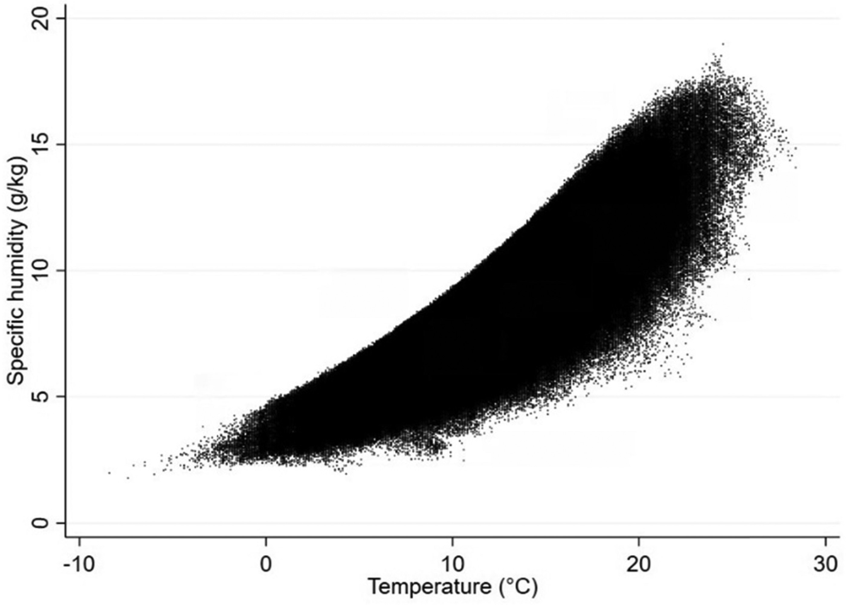
9 PET includes temperature, relative humidity, wind speed, and solar radiation measures. One of the conclusions of the study was that the inclusion of PET is not particularly beneficial. Based on these results, we disregard humidity in most of the analyses. However, we include a test of how humidity affects our baseline results in the Robustness Checks section.
There is evidence that temperature effects are delayed in time, and health effects of temperature accumulate (e.g., [
20]). Several studies have estimated that heat effects are rather immediate and persist three to five days, while cold effects persist for longer, up to 15 days.
21,22 Therefore, studies often contain a lag structure for temperature. Distributed lag models (DLM) are common tools in environmental epidemiology, notably the distributed lag nonlinear model (DLNM). Developed by Armstrong, DLNM is adapted from DLM to include the estimation of nonlinear exposure effects.
23 The method models the exposure–response association in two dimensions, using separate functions for the lag dimension and the predictor. Gasparrini et al. examined temperature-related cause-specific mortality in the United Kingdom between the years 1993–2006 using the DLNM method.
24 They found that all-cause mortality rises by 2.1 percent for each day with a temperature above the 93rd percentile of region-specific yearly temperatures.
24(p56) More than half of the measured mortality was attributable to cardiovascular and respiratory diseases.
24(p56)Another reason to include the lag dimension is to account for the harvesting/displacement effect. Harvesting takes place when the number of deaths peaks as an immediate response to high temperatures, which is partially compensated for by a reduction in mortality in the following period. The effect concerns mainly individuals who are extremely vulnerable and whose deaths are preponed by any additional stress. According to some studies, the initial mortality increases during heat waves are largely driven by the harvesting effect and are offset by a subsequent fall in mortality.
25 Therefore, harvesting needs to be considered when analyzing the causal effects of heat.
Vulnerability to heat stress can be categorized as follows. First, certain population groups might experience increased exposure to heat. This could be true in cities, where the urban heat island effect, or the occurrence of elevated temperatures in urban areas due to paved surfaces, human activities, and energy usage, takes place. Evidence from Sweden shows that the temperatures in the city of Gothenburg can be, on average, 6°C higher during the summer compared to surrounding rural areas.
26 Second, some population groups are more sensitive to heat stress. Several studies report a significantly higher risk of hospitalization and mortality for elderly people, related to both heat waves and cold spells, compared to the prime-age group.
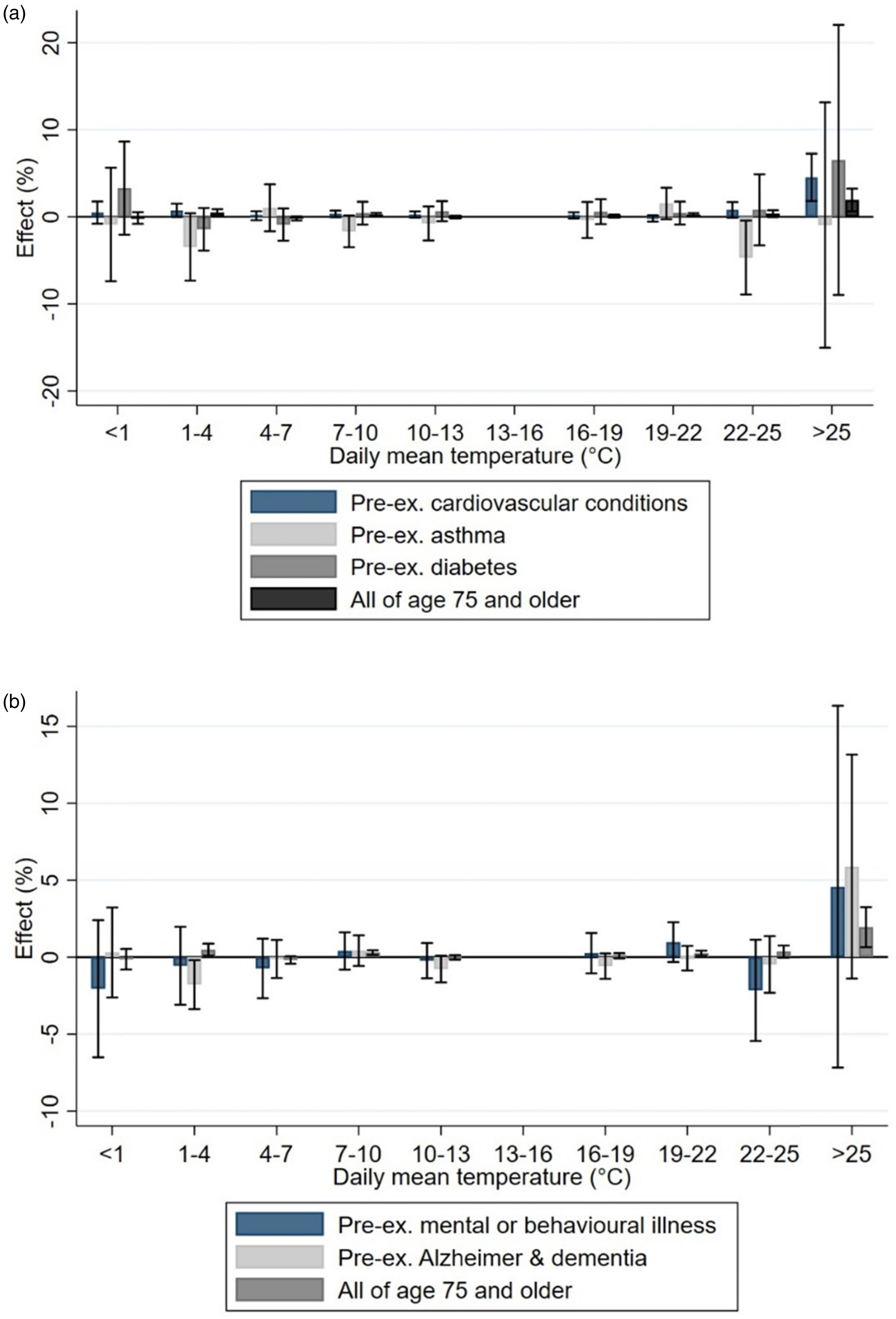
27,28 An aging population typical to the Nordic countries is thus another factor aggravating the effects of heat waves in Finland. Third, heat affects health through different mechanisms, and health effects are likely to channel through specific diagnosis categories in the health care system. Moreover, people with certain pre-existing conditions might be more susceptible to heat-related health effects. According to earlier studies, hospital visits related to asthma are elevated during heat waves.
29 Diabetes has also been reported to elevate the risk of negative health consequences.
30 Some studies have shown that high temperatures cause cardiovascular hospitalization and individuals with pre-existing cardiovascular illness have an elevated risk for morbidity and mortality.
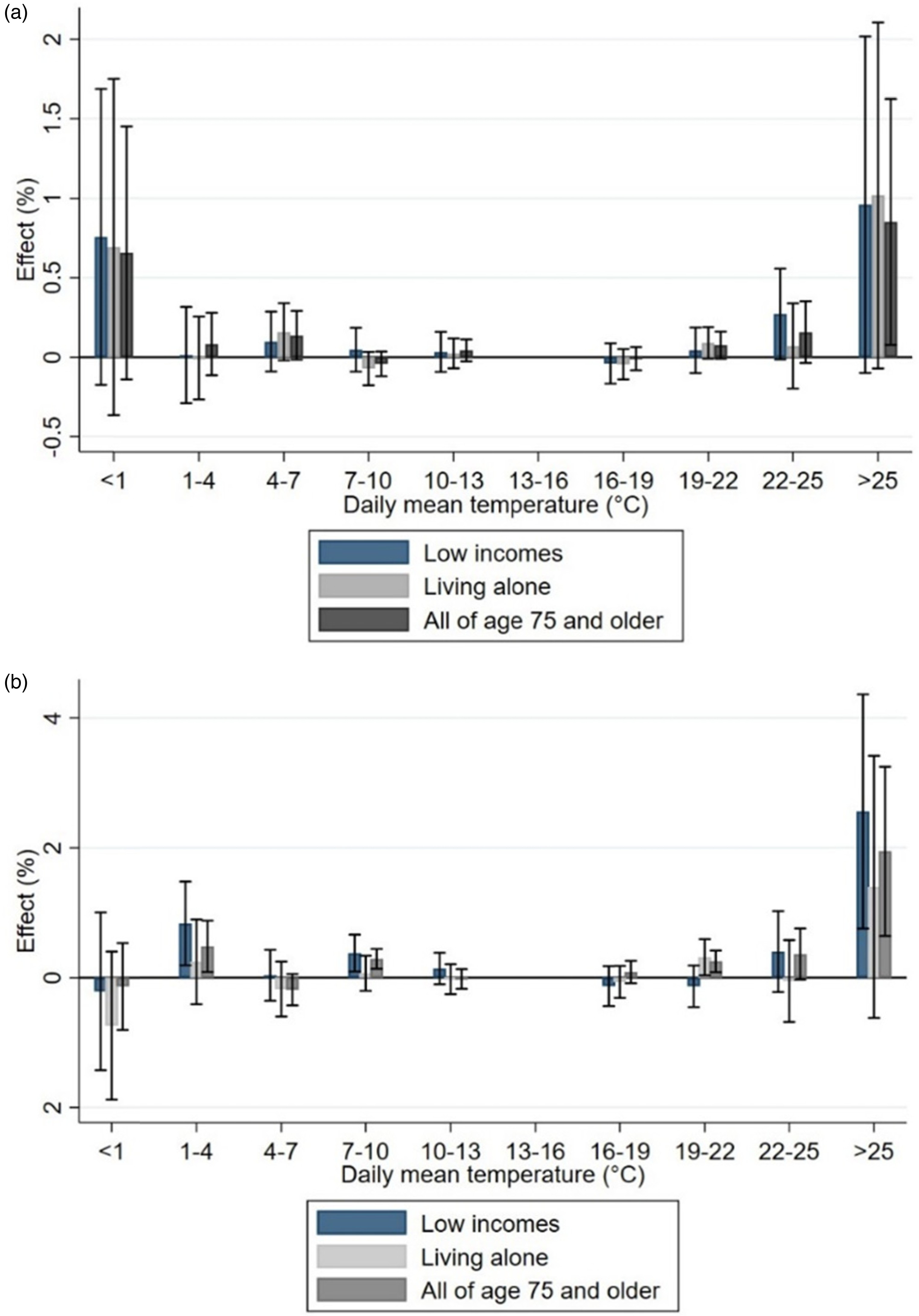
31Higher sensitivity often overlaps with lower adaptive capacity. The degree to which individuals or households can adapt their behavior to heat exposure in the short term is a major determinant of health consequences. For example, there is evidence that elderly population living alone faces larger health risks from heat stress.
32 Not having anybody to take care of oneself might cause symptoms of heat exposure to remain unattended or decrease the use of simple preventive measures such as staying hydrated or opening the windows. History of dementia-related illness is another potential reason for added risk of heat-related mortality and morbidity, due to hindered adaptive capacity. Rocklöv et al. argue that dementia might explain a significant part of heat-related mortality among the elderly population in Sweden.
33 Also, people with low incomes might also be less able to adapt to high temperatures—for example, by investing in air conditioning or relocating. However, there is little evidence on elevated heat vulnerability of groups in lower socioeconomic positions from the developed countries. Gouveia et al. found only little evidence that socioeconomic position would affect the temperature–mortality relationship in Brazil.
34 A study comparing cities in the United States showed that a 10 percent increase in a city's poverty level increased the heat-mortality association by 4.3 percent per a 10°F increase in temperature.
35Data and Research Design
Data
We use register data on the use of specialized health care (HILMO) administered by the Finnish Institute for Health and Welfare, data on individuals’ basic information (FOLK) and causes of death administered by Statistics Finland, and daily weather data administered by the Finnish Meteorological Institute. Individual information is merged by using a unique identifier. Municipal-level daily health outcome counts and daily weather are aggregated to the municipality-month level to form a panel dataset used in the empirical analyses.
The data span from 1998 to 2017 but only the summer months from May to September are included in order to focus on heat effects. This also mitigates the possible confounding effects of the early spring road dust period. We fix the municipality borders to the ones of 2015 throughout the data due to municipal mergers. Some spatial accuracy is lost by doing this, since some weather data are disregarded and replaced with measurements from the parent municipality.
Outcome Variables: Hospital Visits and Mortality
We are interested in two outcome variables: hospital visits and mortality. All health care services in Finland are divided into primary health care and specialized health care. The health care data used in this article consist of public-sector specialized care visits. Our data cover around half of all the outpatient visits in the public sector, as there were 10.8 million outpatient visits in specialized care compared to 9.9 million outpatient visits in primary health care during the year 2019.
36,37 The data include primary symptom diagnosis codes corresponding to the International Classification of Diseases 10th edition (ICD-10) to distinguish between diagnosis groups and a variable to distinguish between acute and other hospital visits.
Seasonalities can be observed when examining all hospital visits—for example, reduced visits during holiday seasons and concentration of scheduled visits on weekdays. Therefore, we include only acute visits that naturally present less seasonality. Examining acute visits also creates a clearer link between the weather exposure and the health outcome. Some seasonalities are also taken into account by the use of fixed effects that restrict only the inter-month variation into the analysis.
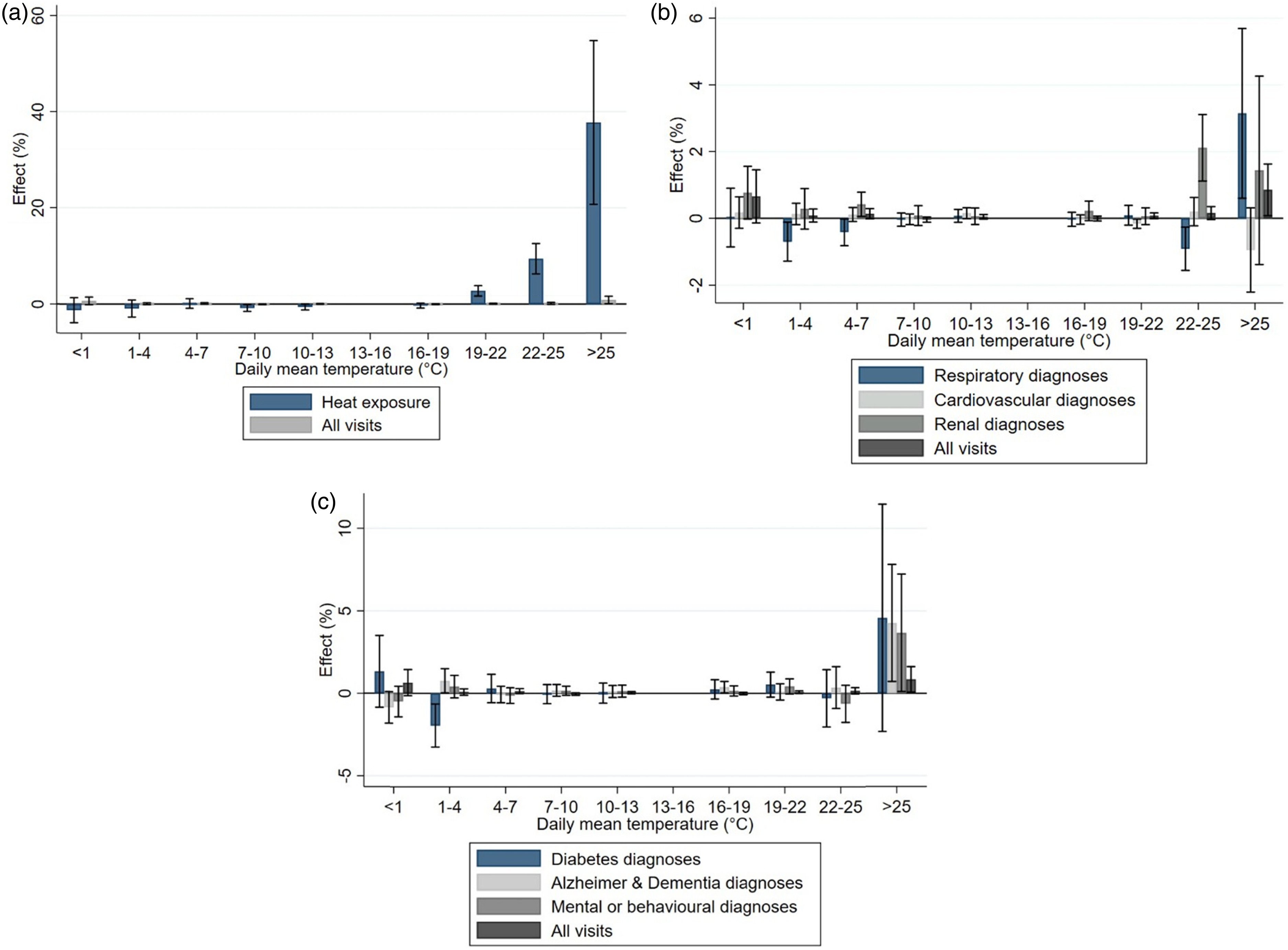
The hospital visits are analyzed cause-specifically using diagnosis codes that are selected based on existing evidence.
38,39 The following ICD-10 diagnosis codes are chosen for the analysis: cardiovascular diseases (I00–I99), respiratory diseases (I60–I69), selected renal diseases (N00–N39), dementia (F00–F03), psychiatric disorders (F04–F99), and diabetes-related diagnoses (E10–E14). Respiratory illness with codes J60–J79 is excluded due to it being caused by inhalation of inorganic substances. Hyperthermia (T67) and exposure to excessive natural heat (X30), are included under the category “heat exposure.”
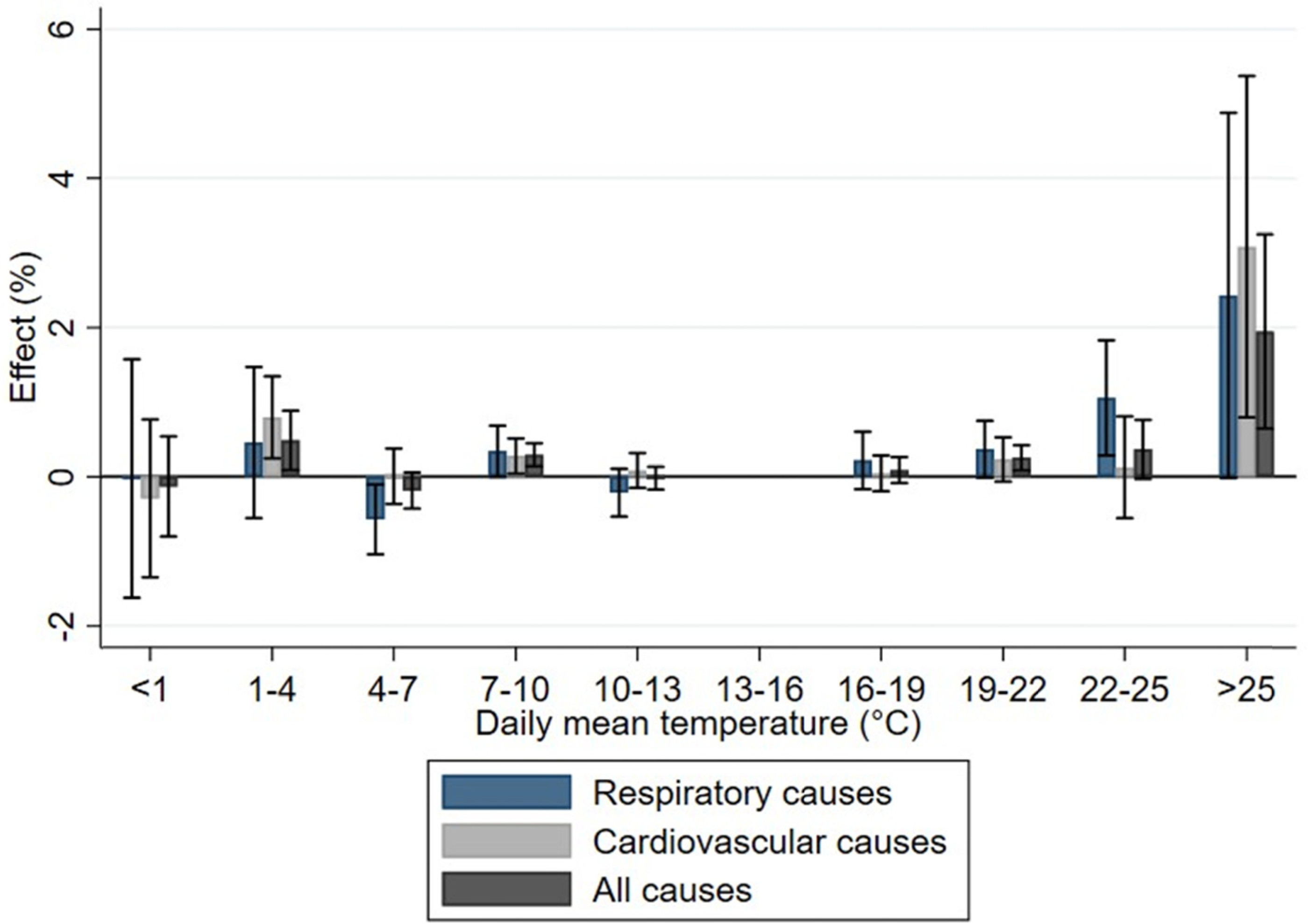
Mortality data contain a main cause of death, an imminent cause of death, and four contributing causes of death. We determine the cause-specific deaths in our data by using both the main and imminent causes of death. We consider separately two of the most common causes of death: cardiovascular causes (I00–I99) and respiratory causes (I60–I69). All outcomes are calculated per 100,000 population, using yearly population estimates calculated using the FOLK data. Summary statistics on the average monthly mortality and hospital visit counts for the study period are presented in
Tables 1 and
2.
Demographic and Socioeconomic Variables
Annual data describing individuals’ basic information is provided by Statistics Finland. Variables used are the municipality number for the place of residence, year, unique identifier, age, disposable income, living arrangement, and a family identifier code. Since the data do not include observations for individuals’ year of death, this information is extrapolated from the previous year for individuals that die during the sample period.
A low-income indicator was constructed based on equivalized family disposable income, a measure taking into account paid taxes and received social transfers. The Organisation for Economic Co-operation and Development modified equivalence scale
40 was used to account for the size and composition of the household: The sum of the family disposable income is divided by a weighted sum of family members, where the first adult of the household is weighted by 1, all following adults by 0.5, and children under 14 by 0.3. Each year, the first quintile of the income distribution—that is, the poorest 20 percent of the population—is defined as the low-income group. We have also created an indicator variable for a living alone status, based on the living arrangement variable.
Data on hospital visits and ICD-10 codes are also used to create indicators of pre-existing medical conditions for each individual. Pre-existing conditions are identified based on an indicator variable that has a value of 1 if an individual has had any acute or non-acute hospital visits during the past five years in the specified diagnosis categories. When using these variables, the first five years of the data are omitted. The diagnoses of interest in determining pre-existing conditions are diabetes, cardiovascular disease, asthma, dementia and Alzheimer's disease, and mental or behavioral diagnoses.
Independent Variables: Weather Data
Weather data are obtained from the Finnish Meteorological Institute (FMI), and the variables used are the municipality number, date, daily mean temperature, and relative humidity. The measures of relative humidity, which contain a component of temperature, are converted into specific humidity (g/m3) using a conventional meteorological formula, after which they are used in the Robustness Checks section.
We have chosen to use daily mean outdoor temperature as the main predictor in the models. The temperature for each municipality in the dataset is calculated based on spatially averaging from the FMI's 10km × 10km gridded dataset. Compared to several studies in which temperature is calculated by averaging between the daily minimum and maximum temperatures, FMI measures are more accurate and less prone to measurement error, as daily mean temperature is calculated by using up to eight daily measures.
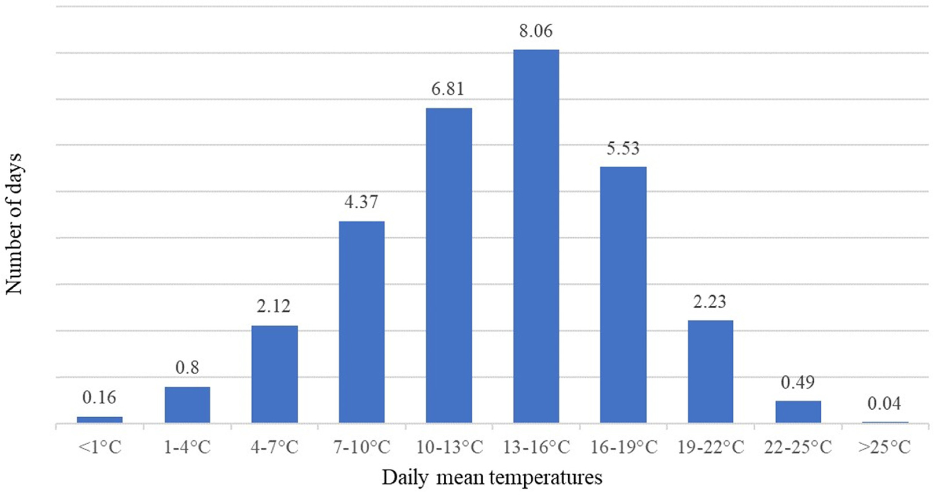
The relationship between temperature and health outcomes is often found to be U-shaped, where negative health outcomes occur at both ends of the temperature distribution. It is essential to take into account the highly nonlinear health effects of temperature. Independent variable binning is a tool to easily model nonlinear effects and is used in several climate economics papers studying the temperature–morbidity effect.
12(p16), 18(p24), 41 The procedure reduces variation but, in turn, parameters can be estimated separately for each category, enabling the modeling of nonlinear effects. The reduction in variation is often overcome by using large data. Aforementioned studies use several decades of daily observations, while our article also uses 20 years of daily measures. An upside of data binning instead of, for example, fitting a polynomial function into the data is that no assumptions of the functional form relationship between the variables are needed, as the association is determined freely by the data. Following this method, we categorize temperature into 10 bins.
Figure 1 shows this categorization and the average distribution of days per month in each bin in the sample. The days in the lowest bin form about 0.5 percent of the municipality-days in the sample and the highest bin about 0.1 percent.
Figure 2 illustrates the spatial distribution of the number of days in the two highest temperature bins.
Empirical Methods
After aggregating the data to the municipality-month level, our empirical model is formalized as follows:
where Y is the monthly sum of hospital visits or mortality per 100,000 population in municipality i, month m, and year y. Y is explained by the sum of days per month in each of 10 different temperature bins
TB. Temperature bin 5, which corresponds to the daily mean temperatures between 13–16°C, is omitted as a reference category. Municipality-year level fixed effects
α(i,y) take into account the differences in trends in the outcome variables between different municipalities and between different years, that could be caused, for example, by differing trends in the local age distribution, health care quality, or any other differences in trends. Month fixed effects
γm take into account seasonality in the outcome variables common to all municipalities and all years—for example, differences in health care use between months. Robust standard errors are clustered at the municipality level in all the regressions due to the plausible correlations between standard errors within municipalities.
Regressions are weighted using the yearly population of each municipality. Using regression weights mitigates the comparability issues between areas that are small and densely populated and areas that are large and sparsely populated by allowing areas to impact the results in relation to their population size.
11(p14) We also conduct the analysis by using the Poisson regression method, first, due to the widespread use of this method in earlier studies
19,34,35,42 and second, due to a concern that especially smaller municipalities might have monthly outcome counts that are Poisson distributed instead of normally distributed. The main specification results using the Poisson fixed-effects regressions are available in the Appendix.
Discussion
In this article, we examined the effects of high temperatures in Finland using unique register data on the total population. Employing linear regression and high-dimensional fixed effects, we analyzed the effects of temperature-days on acute all-cause and cause-specific hospital visits and mortality and examined the effects in various subgroups of the population. Our contribution lies especially in examining health care use alongside mortality, as well as in identifying vulnerable groups. We also introduce a model widely used in climate economics but not yet applied to Finland or other Nordic countries.
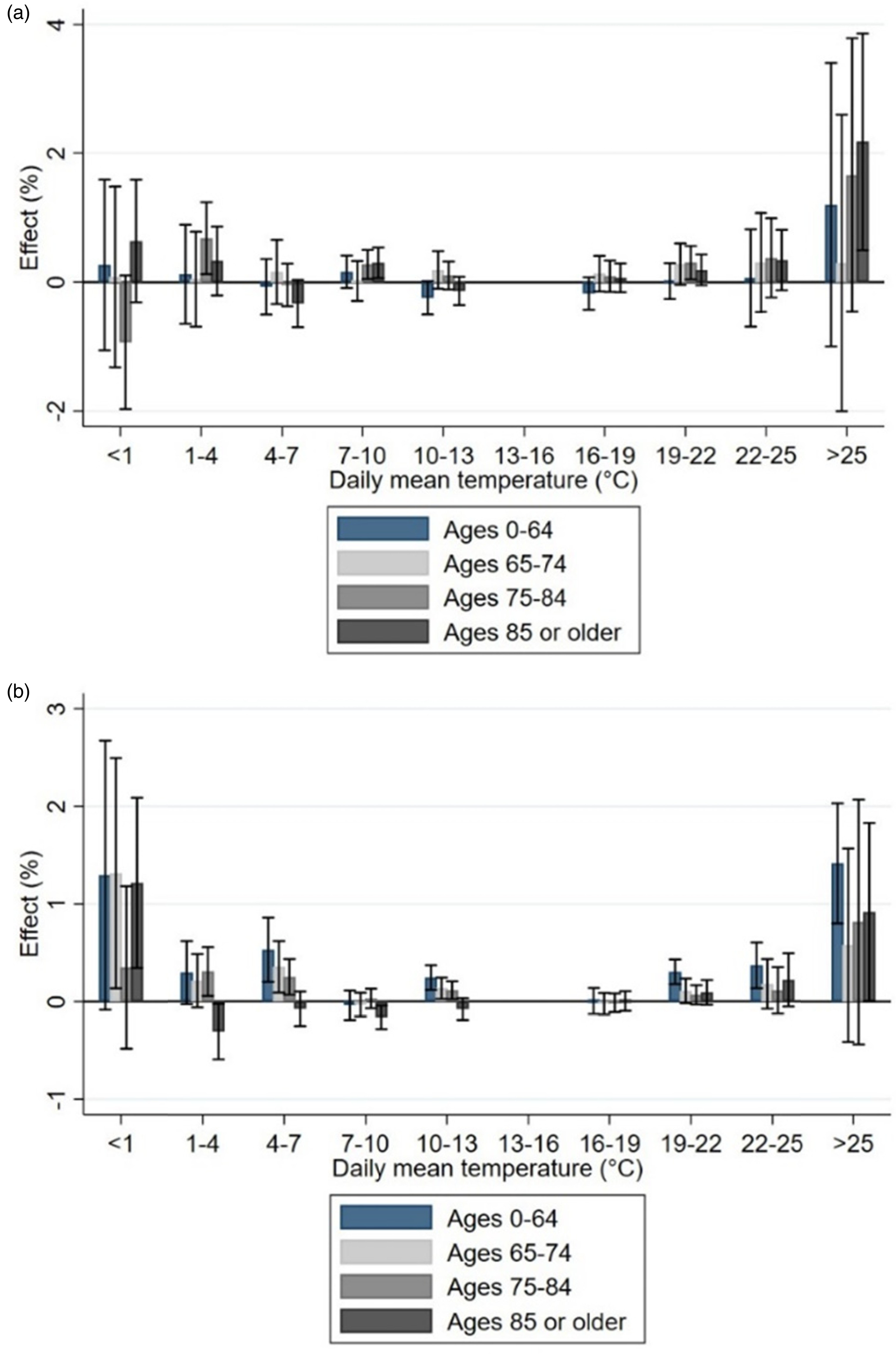
Our results show that the highest temperatures were associated with a clear increase in the number of hospital visits and excess deaths. Relative increases in acute hospital visits but not in mortality were visible for younger age groups, too, perhaps indicating that working-age individuals are not able to protect against heat or indicating vulnerability among young children. In addition, it suggests that the significance of heat effects is underestimated among the working-age population. The finding also shows that using hospital visits as an alternative health indicator (in addition to mortality) can uncover less extreme health consequences that are, nevertheless, important for the functioning of the health care system. While we acknowledge the need to conduct more research on the working-age population and working conditions during heat waves, our main effort was to study effects in more detail among the elderly population.
The effects were indeed strongest among the older population groups as demonstrated by previous literature.
8(p1), 12, 25(p. 600) However, against our expectations, we were in several cases unable to detect an elevated risk among older people with pre-existing medical conditions, which could indicate that individuals in these groups are mostly aware of the health risks connected to heat waves and are prepared to protect themselves. However, individuals with Alzheimer's disease/dementia were one of the groups among which a higher effect on hospitalization and mortality was found. This result is in line with previous literature (e.g., [
33]). From the perspective of designing effective heat alert mechanisms, it is important to note that the individuals most at risk may lack cognitive capacity to react sufficiently. Vulnerability factors should thus incorporate not only physical health dimensions, but also dimensions of cognition. However, we did not find individuals with mental health problems to be at a higher risk.
In addition, low-income elderly people were affected more strongly in terms of mortality and acute hospital visits than all persons 75 or older. This could be related to the overall worse health or lower adaptive capacity among the group. As with dementia, this highlights the weaker coping skills of vulnerable groups. In the future, more research is needed on, for example, the housing conditions and living environment that can protect against negative consequences of high temperatures. For example, evidence from England shows that individuals in the poorest income quintile are four to five times more likely to experience overheating in their homes compared to the richest income quintile.
43Our results are similar in magnitude to the results of some studies, to the extent the analyses are comparable. For example, Barreca estimated that three additional days above 90°F (approximately 32°C) resulted in 0.54 excess deaths per month per 100,000 population in the United States, or a percentage effect of 0.78 percent when reflected against the mean mortality rate.
18(p25) Deschênes and Greenstone estimated that an additional day above 32°C per year increases annual all-cause mortality by 0.11 percent in the United States.
12(p153) Otrachshenko et al. estimated a mortality effect of 0.06 percent for an additional day per year above 25°C in Russia.
41(p295) Our most comparable result for the all-cause mortality effect for the whole population (Table A.2) ranges from 0.3 percent for an additional day in the range 22–25°C to 1.5 percent for days above 25°C. In relation to other studies from Finland, our results on mortality are smaller in magnitude. For example, Ruuhela et al. found an effect on mortality of 16 percent at a daily mean temperature of 24°C, using the DLNM method and daily level analysis.
44 Kollanus et al. defined heat wave as a period in which the daily mean temperature exceeds the 90th percentile of that from May to August during the years 2000–2014, or about 20°C.
8(p1) They found average mortality effects of 6.7 percent in the age group 65–74 and 12.8 percent during all heat wave days in the age group 75 or older.
8(p1)As a limitation of our study, the way in which causes of death are reported differs from the broader set of diagnoses reported in the data on hospital visits. Causes of death are more concentrated, with the two most common diagnoses being cardiovascular and cancer diagnoses, and thus less information is available on the exact causes. In practice, heat-related morbidity by certain causes is not represented in the causes of death statistics, and heat-related mortality by some causes is not represented in the morbidity statistics. This was visible for cardiovascular diseases: Mortality from these causes increased, but not hospital visits. In conclusion, multiple indicators of health outcomes should be used in studying the health effects of temperature. Since this article only includes specialized care visits, there might also be some selection implications. Visits to occupational health care or private health care are not reported in our data.
Another concern about the causal inference in this study is the increase in traveling and the common Finnish habit of spending time at summer cottages during the summer, which means that people are away from their home municipalities. Unfortunately, the hospital discharge register data only includes the home municipality of the individual, instead of the municipality where the visit took place. This hampers the causal analysis for obvious reasons. In addition, individuals with health problems might seek respite in the cooler countryside during heat waves, while individuals might be in very unequal positions in their abilities to do so.
Conclusions
Deadly heat waves have alerted governments and public health officials to react to the negative health consequences of global warming.
45 Climate change has also increased the likelihood of heat waves in Finland, where the population is used to mild temperatures and where cold temperatures have previously been viewed as a larger risk for public health.
7(p452) In the past decades, temperatures have been rising in the northern countries more than the global average.
2(p1) The change necessitates new research in this geographical context to identify vulnerable groups and to adapt the health care sector to protect public health.
It is possible that in the long term, the population can adapt to higher temperatures. The gradual unfolding of climate change will allow for adaptation measures in the long term that are impossible to predict. Folkerts et al. found that the minimum mortality temperature has increased in the Netherlands during the years 1995–2017.
46 In addition, Barreca shows that warmer counties in the United States were less susceptible to high temperatures and humidity levels compared to cold counties.
18(p28) It is unclear whether this acclimatization is due to physiological, infrastructural, behavioral, or technological adaptation. Further research on the acclimatization across time and the differences in vulnerability across different parts of northern hemisphere would be valuable. The good news is that Finland and many other wealthy countries in the North are better able to adapt their infrastructure and health care systems compared to poorer countries elsewhere.
Short-term adaptation measures against heat can consist of, for example, accessing cooler areas or spaces, using air conditioning, or avoiding physical stress. Long-term adaptation can include, for example, migration and redesign of urban areas and construction methods. Farhadi et al. examined mitigation possibilities of the urban heat island effect and found that increasing urban vegetation cover can significantly mitigate the effect.
47 Another important form of adaptation takes place at the community level, and policy measures are also needed to protect public health, for example, through education, preventive health care, and heat wave warning systems.
45Paavola has pointed out that relying on individual-level behavior change and preparedness might result in increased health and social inequality, since the uptake of these measures can be highly selective.
48 Indeed, our results show that low-income individuals and individuals with dementia are at higher risk of negative health consequences. The lack of financial resources and weakened cognitive capacity might hamper the effectiveness of policies targeted at individuals. Therefore, efforts should be put in studying the effectiveness of adaptation policies and interventions and their impact on different population groups. Various dimensions of vulnerability need to be taken into account, including socioeconomic factors and mental or cognitive functioning. At the same time, research projecting local and national health consequences of climate change and related costs in the health and social care sector is needed.