	New content
Statistical Modelling

Open access

Research article

First published online February 9, 2026

D-optimal designs for beta binomial regression

Klazien de Vries https://orcid.org/0009-0007-9302-1562 [email protected], Marieke E. Timmerman https://orcid.org/0000-0003-1579-6964, and Casper J. Albers https://orcid.org/0000-0002-9213-6743View all authors and affiliations

OnlineFirst

https://doi.org/10.1177/1471082X261416637

Abstract
1 Introduction
2 Methods
3 Results
4 Sensitivity
5 Discussion
Acknowledgements
Declaration of Conflicting Interests
Funding
ORCID iDs
References
Supplementary Material

PDF/EPUB

Abstract

Optimal designs describe the sampling distributions that achieve most efficient estimation. In this study, we apply optimal design theory to find optimal designs for the beta binomial (BB) regression model, where both location and dispersion are functions of a predictor. A major application of the BB regression model is in psychological test norming, where the location and the dispersion of test scores can be age dependent. Motivated by this context, we derive and characterize locally D-optimal designs for the BB regression model. In a practical example, we consider the designs’ sensitivity to specification of model parameters, model form and optimality criterion. The designs were found to be relatively robust to these effects and thus show promise for practical implementation. However, more research is needed to investigate the suitability of the D-optimality criterion for psychological test norming and to extend the designs to be globally optimal.

1 Introduction

In the theory of optimal design of experiments, an optimal design informs the researcher which points to sample to achieve the most efficient estimation. More specifically, the researcher first assumes a statistical model connecting the response variable to the predictor(s) in a design region, after which a design can be derived that is optimal according to a suitable optimality criterion. The implementation of an optimal design can improve efficiency and reduce costs.

While optimal design theory has traditionally been used in industrial applications (see Goos and Jones, 2011, for example), it has also been gaining traction in the social sciences (see Berger and Wong, 2009). A particular field in the social sciences that could benefit from optimal design theory is psychological test norming. The goal of psychological test norming is to derive normed scores (e.g., percentiles, normalized z-scores, normalized intelligence quotient (IQ) scores) for a psychological test or questionnaire, typically used in developmental or neuropsychological assessment. Normed scores express an individual’s test performance relative to a reference population, for example, individuals of the same age in the same country. To derive normed scores, first, a sample of test scores and relevant predictor(s) is collected from the population. Next, the test score distribution, conditional upon the predictor(s), is estimated from a statistical model. The conditional test score distribution is then used to derive normed scores.

A popular statistical model for psychological test score data is the beta binomial (BB) regression model (see e.g., Timmerman et al., 2021; Urban et al., 2024). The BB regression model is well-suited for discrete, bounded count data, such as the number of correct responses out of a fixed number of test items. A BB model extends the binomial model by allowing the success probability to vary across individuals according to a beta distribution. This enables modelling the overdispersion that can arise from unobserved heterogeneity in individuals’ latent abilities. In BB regression models, both the mean (μ) and dispersion (σ) parameters are regressed against functions of relevant predictor(s), making the model part of the larger class of Generalized Additive Models for Location, Scale and Shape (GAMLSS; Rigby and Stasinopoulos, 2005). In psychological test norming, the BB regression model is typically used to describe how both the expected score and its dispersion change as smooth functions of age, while the total number of test items is fixed and known (e.g., Timmerman et al., 2021; Urban et al., 2024). Beyond psychology, BB regression has been applied in various fields, including microbiology (Martin et al., 2020), toxicology (Slaton et al., 2000) and genomics (Dolzhenko and Smith, 2014). More generally, the BB regression model is suitable when the response represents a bounded count variable exhibiting extra-binomial variability and when both the mean and dispersion parameters are expected to vary with relevant predictors.

In this article, we derive locally D-optimal designs for the BB regression model, thus applying the theory of optimal design of experiments in the psychological test norming context. The designs we derive are D-optimal designs, meaning that they minimize the generalized variance of the estimated model parameters. Furthermore, the designs are locally optimal, not globally optimal, because they are dependent upon the specification of the model parameters. This research can be viewed in the light of three separate lines of research, two from the field of optimal designs of experiments and one from the field of psychological test norming.

First, this research expands research into optimal designs for parametric models where multiple parameters depend upon the predictor(s). Following the convention in psychological test norming, we refer to such models as GAMLSS models (Rigby and Stasinopoulos, 2005), but note that Atkinson et al. (2014) introduced similar models in an optimal design context under the name ‘generalized regression models’. Optimal designs for GAMLSS models have not been studied as extensively as optimal designs for conditional mean models, such as (generalized) linear regression models (see e.g., Fedorov and Hackl, 2012; Dean et al., 2015). To the best of the authors’ knowledge, the only GAMLSS models for which optimal designs have been studied are the normal regression model with parametrized mean and variance (Atkinson and Cook, 1995; Downing et al., 2001) and the beta regression model (Wu et al., 2005). More recently, Atkinson et al. (2014) have provided a general framework for deriving optimal designs for GAMLSS models for several two-parameter distributions, including the gamma regression model.

A related contribution is provided by Cole (2021), who studies optimal sample size and sample composition for GAMLSS-based growth chart construction across four empirical datasets. His approach aims to make the precision of the estimated z-scores as uniform as possible across age by sampling uniformly on a transformed age scale and selecting the transformation parameter accordingly. However, as growth data are typically continuous and unbounded, the approach does not address bounded-count outcomes that can arise in psychological test norming.

Second, the current research extends a more specific line of research on optimal designs using the BB distribution. In a medical context, Arnoldsson (2003) considered locally D-optimal designs for the BB logistic regression model, where only μ is a function of the predictor. The current research extends upon Arnoldsson (2003) by additionally allowing the dispersion parameter σ to depend upon the predictor.

Third, this research extends previous research into optimal designs for psychological test norming by Innocenti et al. (2023). Innocenti et al. (2023) derived locally and globally optimal D-optimal designs for linear regression models with normally distributed homoscedastic residuals. A notable feature of continuous D-optimal designs for these particular models is that they are also G-optimal (see Kiefer and Wolfowitz, 1960). G-optimal designs minimize the maximum sampling variance of the response. Under the assumed model, G-optimal designs also minimize the maximum sampling variance of the normed score estimates, which is of key interest in psychological test norming. The current research extends this line of research by deriving D-optimal designs for a more complicated test score model that can handle discrete, non-normal and heteroscedastic test scores.

This article is organized as follows. First, in Section 2, we describe the BB regression model in detail, give an introduction to optimal design theory and describe the numerical procedure we used to derive optimal designs. Hereafter, in Section 3, we present and characterize the resulting optimal designs for the BB regression model, using known optimal designs for related models to aid interpretation. Next, in Section 4, we apply the D-optimal designs in a practical example, investigating concerns regarding sensitivity of the designs to choice of model parameters, model form and optimality criterion. We end with a discussion of the results.

2 Methods

2.1 Beta binomial regression

In BB regression for psychological test norming, individuals’ test scores Y_i follow a BB distribution with the following probability density function (following the parametrization in Stasinopoulos et al., 2017)

p (y_{i} | μ, σ, n) = (\begin{matrix} n \\ y_{i} \end{matrix}) \frac{Γ (y_{i} + \frac{μ}{σ}) Γ (n - y_{i} + \frac{1 - μ}{σ}) Γ (\frac{1}{σ})}{Γ (\frac{μ}{σ}) Γ (\frac{1 - μ}{σ}) Γ (\frac{1}{σ} + n)} .

The parameter μ ∈ (0, 1) is related to the probability of answering a test item correctly and σ > 0 is a dispersion-type parameter. The parameter n > 1 represents the total number of items in the test and is assumed to be fixed across individuals. The mean and the variance of the BB distribution are

\begin{matrix} E [Y] = n μ, \\ Var (Y) = n μ (1 - μ) [1 + (n - 1) \frac{σ}{σ + 1}] . \end{matrix}

(2.1)

The variance of the BB distribution equals the variance of the binomial distribution, multiplied by an overdispersion factor. Larger values of n and σ result in more overdispersion in the test scores. Instead of σ, some authors use the intra-class correlation coefficient ρ = σ/(σ + 1) (e.g., Arnoldsson (2003)) to characterize the over-dispersion. The intra-class correlation coefficient measures the correlation between Bernoulli trials in the underlying mixture representation, where Y_i is viewed as a binomial(n, p_i) random variable with p_i ∼ beta(α, β). In the limit σ → 0 (i.e., ρ → 0) the variance of the BB distribution reduces to the binomial variance nμ(1 − μ). On the other hand, when σ → ∞ (i.e., ρ → 1) it approaches n² μ(1 − μ), the variance of a Bernoulli random variable supported on {0, n}.

The dependency of the location μ and dispersion σ on a predictor

x_{i} \in ℝ

, such as age, is modelled through the link functions

\begin{matrix} logit (μ) = α^{T} f (x_{i}), \\ \log (σ) = β^{T} g (x_{i}), \end{matrix}

where

α^{T} = (α_{1}, α_{2}, \dots, α_{p}) \in ℝ^{p}

and

β^{T} = (β_{1}, β_{2}, \dots, β_{q}) \in ℝ^{q}

and f(x) and g(x) are vectors of linearly independent continuous functions. Furthermore, let θ = (α, β) denote the vector of unknown parameters and m = p + q the total number of unknown parameters.

2.2 Locally optimal designs

In this section, we briefly outline the theory of optimal design as applied to the BB regression model. General introductions to the topic can be found in Fedorov and Hackl (2012) and Atkinson et al. (2007), with a comprehensive overview of the field provided by Dean et al. (2015).

Let the response variable be distributed as Y ∼ p(y; x, θ), where θ ∈ Θ is the unknown parameter vector. For the BB regression model, θ = (α, β) combines the regression parameters for the mean and the dispersion. We assume that the design variable

x \in X

is univariate, typically representing a single continuous predictor such as age in many psychological test norming applications. Similarly, we assume that the response y is also univariate, representing a single test score. For simplicity, we focus on this univariate predictor and univariate response case, although the approach can be extended to multivariate predictors and/or responses. A design ξ consists of design points in the design region

x_{i} \in X, i = 1, \dots, k

, each assigned a design weight w_i > 0 with

\sum_{i} w_{i} = 1

. The design can be represented as

ξ = \{\begin{array}{l} x_{1}, x_{2}, \dots, x_{k} \\ w_{1}, w_{2}, \dots, w_{k} \end{array}\} .

To simplify finding D-optimal designs, we focus on continuous (large-sample; approximate) designs, where the weights can be any positive real numbers summing to one, unlike exact designs that require integer-valued replications. Guidelines on normed score construction typically involve normative samples with hundreds to thousands of observations (see e.g., Evers et al., 2009), hence this continuous approximation is appropriate.

An optimal design is a design that holds maximal information on the parameter vector θ, in terms of the Fisher Information Matrix (FIM). The FIM for a single design point x_i is defined as

M_{i} (θ; x_{i}) = - E_{Y} [\frac{\partial^{2} l (Y; x_{i}, θ)}{\partial θ \partial θ^{T}}],

where ℓ(y; x_i, θ) denotes the log-likelihood of BB regression model.

Unlike in generalized linear models, the FIM in BB regression cannot be written as a simple scaled outer product (see e.g., Atkinson and Woods, 2015) because the mean and dispersion parameters affect the likelihood in a nonlinear way. As a result, the FIM for the BB regression model contains cross-derivative terms between the mean and dispersion regression parameters.

M_{i} (α, β; x_{i}) = - E_{Y} [\begin{matrix} \frac{\partial^{2} l}{\partial α \partial α^{T}} & \frac{\partial^{2} l}{\partial α \partial β^{T}} \\ \frac{\partial^{2} l}{\partial β \partial α^{T}} & \frac{\partial^{2} l}{\partial β \partial β^{T}} \end{matrix}],

where the dependency of the log-likelihood function on y, x_i and θ was dropped for ease of notation. The full derivation of the FIM for the BB regression model is provided in the supplementary material.

The overall FIM of a design ξ is now a weighted sum of the FIMs in the design points:

M (θ; ξ) = \sum_{i = 1}^{k} w_{i} M_{i} (θ; x_{i}) .

The inverse of the FIM is proportional to the asymptotic covariance matrix of the maximum likelihood estimator under mild regularity conditions (see e.g., Ferguson, 2017). Hence, maximizing the information in a design can be thought of as minimizing the asymptotic variance of the maximum likelihood estimates.

A common measure of design optimality is the D-optimality criterion (see e.g., Atkinson et al., 2007, chapter 10), which seeks to maximize the determinant of the FIM:

ξ^{*} = \arg \max_{ξ} \det [M (θ; ξ)],

thus minimizing the volume of the confidence ellipsoid for the maximum likelihood estimates of θ.

Because the BB regression model is nonlinear, the FIM depends on the unknown parameter vector θ. Consequently, the resulting optimal designs are parameter-dependent and must be computed for a prespecified value θ₀. Designs obtained in this manner are called locally optimal designs. In contrast, globally optimal designs are optimal over a range of plausible parameter values Θ₀ ∈ Θ. There are several ways of deriving globally optimal designs, for example using Bayesian, sequential or maximin approaches. Deriving globally optimal designs for the BB regression model is beyond the scope of this article; see Atkinson and Woods (2015) for further discussion.

Figure 1 Sensitivity function ψ(*x, ξ*^*) of a D-optimal design.

2.3 Numerical procedure

In the supplementary material, we derive the FIM for the BB regression model. The resulting FIM involves expectations of several digamma and trigamma functions, which makes the analytical derivation of D-optimal designs intractable. Therefore, we rely on numerical procedures to obtain locally D-optimal designs.

For convex optimality criteria such as D-optimality, the optimality of a design can be verified through its sensitivity function (see e.g., Fedorov and Hackl, 2012)

ψ (x; ξ) = tr [M (θ; x) M^{- 1} (θ; ξ)],

where M(θ; x) is the FIM under a single-point design at x and M(θ; ξ) is the FIM under design ξ. Intuitively, ψ(x; ξ) measures the potential information gain of adding design point x to ξ; if ψ(x; ξ) exceeds m, the design can still be improved by assigning more weight to x. The Kiefer–Wolfowitz equivalence theorem (Kiefer and Wolfowitz, 1960) states that, for a D-optimal design ξ^*, the maximum sensitivity over the design region

X

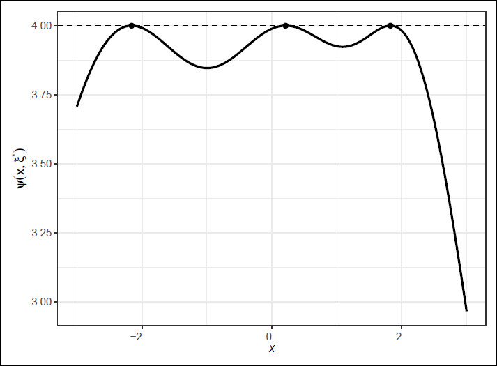
equals the number of model parameters m and this maximum is attained precisely at the design points of the design. This theorem hence provides both a criterion for convergence and a diagnostic tool to assess the optimality of a numerical solution. Figure 1 illustrates this theorem, showing the sensitivity function ψ(x, ξ^*) of the D-optimal design ξ^* of a BB regression model with linear effects of age in μ and σ (α = [0, 1], β = [−2.5, 0.6]). The horizontal dotted line represents the number of parameters m = 4 and the black dots indicate the location of the design points.

To numerically obtain optimal designs, we used a hybrid algorithm akin to the ‘cocktail algorithm’ by Yu (2011). This hybrid algorithm combines ideas from coordinate exchange and multiplicative algorithms, hence we refer to it as the CE+MA algorithm. Coordinate exchange algorithms (e.g., Meyer and Nachtsheim, 1995; Dean et al., 2015, Chapter 21.4.2) iteratively adjust individual design points to locally improve the D-optimality criterion while holding other points fixed. Multiplicative algorithms (e.g., Pronzato and Pázman 2013, Chapter 9; Dean et al. 2015, Chapter 21) update design weights proportionally to their local sensitivities.

The CE+MA algorithm iteratively improves a candidate design by alternating between coordinate exchange and a multiplicative update. To improve numerical stability and convergence, small weights are pruned and nearby points are merged after each iteration, similar in spirit to the approach by Yu (2011). The algorithm terminates when the sensitivity criterion is met.

To further enhance robustness, an adaptive implementation was used that automatically adjusted tuning parameters (e.g., damping and iteration limits) and reinitialized non-converged runs, ensuring stable convergence across diverse parameter configurations. In practice, the adaptive CE+MA algorithm was found to converge sufficiently across a wide range of BB regression settings, achieving numerical accuracy up to 10⁻⁴ and often much lower (10⁻⁸). The complete and annotated R implementation is provided in the supplementary material.

3 Results

Before we present and characterize D-optimal designs for the BB regression model, we first recap existing results on related models, namely the logistic regression model and the BB logistic regression model. For the canonical logistic model with a single continuous predictor and binomial response, the optimal designs take the form of equally weighted two-point designs, placed symmetrically around μ = 0.5, at predictor values corresponding to μ = 0.176 and μ = 0.824 (see e.g., Atkinson and Woods, 2015). Note that design points where the mean response probability is μ = 0 or μ = 1 are uninformative of the model parameters.

For the BB logistic regression model, D-optimal designs are given by Arnoldsson (2003). Although Arnoldsson (2003) uses the intra-class correlation coefficient to characterize the dispersion, this BB logistic regression model can be thought of as a BB regression model with a constant, but parametrized, dispersion σ. For a range of dispersion parameters and binomial denominators n of 16 or less, they found that D-optimal designs for the BB logistic regression model also take the form of a symmetric, two-point design, centred around μ = 0.5. Compared to the logistic regression model, design points were moved inwards towards μ = 0.5, more so for large dispersion and small binomial denominators.

It should be noted here that the optimal designs in Arnoldsson (2003) are derived in a medical dose-response context. Here, the binomial denominator n is interpreted as the number of people who are administered a certain dose x of a drug. This number is typically quite small and can vary per dose. In the context of psychological test norming, the binomial denominator n pertains to the number of items, that is, the test length. This is typically larger than 16 and assumed fixed over individuals. For small n, our results corresponded to the D-optimal designs described in Arnoldsson (2003), but for larger n, we found some interesting deviations from the general D-optimal designs which are worth mentioning below.

Using the numerical procedure described in Section 2.3, we constructed D-optimal designs for several BB regression models. Because the BB regression model differs from the BB logistic regression model already investigated by Arnoldsson (2003) in the predictor dependency of σ, our main interest was the effect of the non-constant dispersion σ on the optimal designs. However, we additionally describe some results for the BB logistic regression model with constant dispersion because we found a different form for some D-optimal designs for larger values of n. We investigated optimal designs for relatively common test lengths of n=25, 50 and 100 items and added the more extreme n = 5 and n = 250 for theoretical comparison.

Figure 2 Random samples and D-optimal designs for BB logistic regression models.

3.1 BB logistic regression in psychological test norming

First, we consider the BB logistic regression model, with link functions

\begin{matrix} logit (μ) = α_{0} + α_{1} x, \\ \log (σ) = β_{0}, \end{matrix}

where we fixed α₀ = 0, α₁ = 1 and investigated several values of β₀ ∈ {−5, −4.95, …, 5}. This range of the dispersion parameter, β₀, corresponds approximately to examining intra-class correlation coefficients from near 0 to nearly 1. This is similar to the investigated range in Arnoldsson (2003), but our n ∈ {5, 25, 50, 100, 250} includes much larger values.

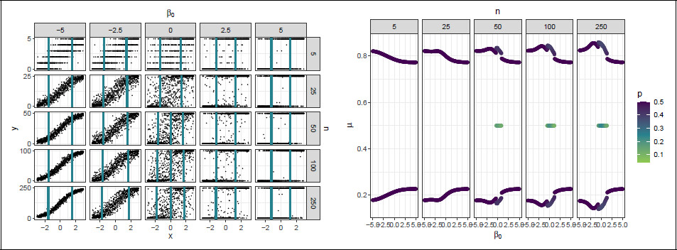
For some selected values of β₀ ∈ {−5, −2.5, 0, 2.5, 5} and all values of n, Figure 2a depicts random samples (N = 1 000), drawing from a uniform distribution for x and generated from their corresponding BB logistic regression models, thus illustrating the investigated models. The vertical lines represent design points from the D-optimal designs. Figure 2a depicts how the value of β₀ affects the test score dispersion. Lower values of β₀ correspond to a near-binomial dispersion and for higher values of β₀, Figure 2a shows that the test scores tend to the extremes, close to a Bernoulli random variable with outcomes in {0, n}. Both observations are in line with the limits for the test score variance of the BB distribution in Equation 2.1.

For each combination of β₀ and n, the corresponding D-optimal designs are displayed in Figure 2b. Design points are represented in terms of their corresponding mean response probabilities μ. Because not all designs were equally weighted, Figure 2b additionally depicts the design probabilities of the design points.

For lower values of β₀, the designs tend to the optimal designs for the logistic regression model. For small values of n, the designs correspond to the findings in Arnoldsson (2003); the D-optimal designs are two-point designs, symmetric around μ = 0.5, with design points moving inwards as the overdispersion increases. This inward shift reflects the movement of the design points toward regions of greater test-score variance (which attains its maximum at μ = 0.5), thereby improving the precision of the estimation of β₀.

For larger values of n, the design points first move outward for centre values of β₀ before shifting inward again for larger values of β₀. Greater separation of the design points improves the precision of the estimation of α₁. It could be that the outward shift only occurs for larger n because the test scores are less concentrated near the 0 and n boundaries and thus extreme design points are more informative than for smaller n.

For some values of β₀, an additional internal design point is placed at μ = 0.5 and the external design points are moved even further outward. For larger n, the range of β₀ for which the internal design point is placed extends and its design probability increases. For large values of β₀, the design points tend to μ = 0.227 and μ = 0.772 for all n.

3.2 BB regression

Next, we consider the BB regression model, where σ now also depends upon the predictor x

\begin{matrix} logit (μ) = α_{0} + α_{1} x, \\ \log (σ) = β_{0} + β_{1} x . \end{matrix}

For the BB regression models, we fixed α₀ = 0, α₁ = 1 and β₀ = −2.5 and varied β₁ from {−1, −0.95, 0.9 …, 1}. These values β₀ and β₁ for the dispersion β₀ were informed by inspecting some commonly occurring values β for subtests of the third Schlichting Language Test (Schlichting et al., 2025).

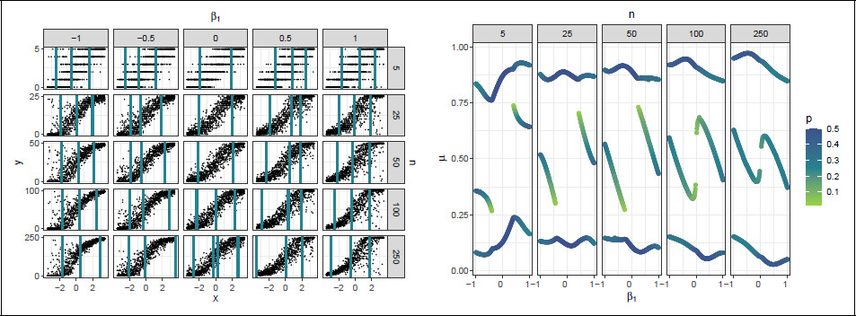
Random samples generated from BB regression models with selected values of β₁ = −1, −0.5, 0, 0.5 and 1 are depicted in Figure 3a, for all values of n. It can be seen in this figure that the dispersion in the response now varies over design region. Negative values of β₁ result in a relatively large dispersion for negative values of x and low dispersion for positive x and vice versa for positive values of β₁. The difference in dispersion over the design region increases as the absolute value of x or β₁ increases.

For each combination of β₁ and n, Figure 3b portrays the D-optimal designs. The design points of the optimal designs are again represented in terms of μ. From Figure 3b, it can be seen that the D-optimal designs for the BB regression model are asymmetric two-point or three-point designs. For small |β₁|, where the dispersion is approximately constant, the designs are equally weighted two-point designs. As |β₁| increases, the designs become increasingly asymmetric and the design points shift away from regions of high dispersion where responses are highly concentrated near 0 or n. This shift reflects a trade-off between maximizing information on the location parameter μ, which favours regions of moderate variability and the dispersion parameter σ, which is best estimated from regions with large changes in overdispersion. The asymmetry in the designs is more pronounced for larger values of n, where differences in response variability across μ are larger. In summary, these D-optimal designs reflect a compromise between regions that are informative for both the mean and dispersion parameters.

Figure 3 Random samples and D-optimal designs for BB regression models.

It should be noted that D-optimal designs for the BB regression model often contain fewer distinct design points than there are model parameters. Some designs include only two points to estimate three or four parameters (see also Atkinson and Cook, 1995; Arnoldsson, 2003), which would be impossible for (generalized) linear regression models. For GAMLSS models, however, this is feasible because the variance can still be estimated through replicated observations at the same design points. Consequently, the minimal number of design points corresponds to what is strictly necessary to estimate the linear predictor in either μ or σ.

4 Sensitivity

Before the D-optimal designs for the BB regression model can be properly implemented, there are still a few issues that need to be addressed. First, because the D-optimal designs are only locally optimal, they are sensitive to the assumed statistical model, both in model parameters and included predictors. Second, the D-optimality criterion we use is aimed at parameter estimation and is not specifically tailored to normed score estimation, where the variance of the normed scores is of main interest. Unlike the designs for linear regression models in Innocenti et al. (2023), the D-optimal designs for BB regression do not necessarily minimize the maximum variance of the normed scores.

In this section, we illustrate and investigate these issues in a practical example. We will consider the sensitivity of the D-optimal designs with respect to model parameters, model form and optimality criterion. As a practical example, we consider empirical test data from the Schlichting Language Test (Schlichting et al., 2025). The particular subtest concerns sentence development in Dutch and Flemish children aged 2–7, and test scores ranged from 0 to n = 36.

4.1 Sensitivity to parameter choice

The D-optimal designs depend upon the prespecified parameter vector θ. In this subsection, we investigate how changes in θ affect the performance of the resulting optimal designs. Suppose that the true BB regression model is given by

\begin{matrix} logit (μ) = 0.01 + 1.04 x - 0.63 x^{2} + 0.76 x^{3} \\ \log (σ) = - 2.65 + 1.06 x, \end{matrix}

where x ∈ [−1, 1] represents a scaled age variable and the maximum test score n = 36. This model was estimated from the Schlichting data and selected using the free order model selection procedure (Voncken et al., 2019) and fitted using the R package GAMLSS, version 5.4-12 (Rigby and Stasinopoulos, 2005).

Table 1 Model parameters, optimal designs and D_def for three models, with θ^*, θ₁ and θ₂ the true, lower bound and upper bound model parameters.

Model	θ	Optimal design ξ_θ	D_def
θ*	α = (0.01, 1.04, −0.63, 0.76) β = (−2.65, 1.06)	$\{\begin{matrix} - 1 & - 0.48 & 0.36 & 1 \\ 0.24 & 0.24 & 0.22 & 0.30 \end{matrix}\}$	1.000
θ1	α = (0.01, 0.52, −0.32, 0.38) β = (−1.33, 0.52)	$\{\begin{matrix} - 1 & - 0.50 & 0.42 & 1 \\ 0.27 & 0.23 & 0.21 & 0.29 \end{matrix}\}$	1.009
θ2	α = (0.02, 1.56, −0.95, 1.14) β = (−3.98, 1.59)	$\{\begin{matrix} - 0.94 & - 0.36 & 0.33 & 1 \\ 0.20 & 0.24 & 0.24 & 0.32 \end{matrix}\}$	1.078

We will follow the approach in Wu et al. (2005) to investigate the sensitivity of the optimal design to the specified model parameters. As a first step, we assume that the model parameters are known with a relative error of 50%, resulting in a lower and upper bound for each model parameter. For example, the lower and upper bounds for α₁ = 1.04 are 0.52 and 1.56. We then considered all the 3⁶ = 729 models resulting from a fully crossed design of the model parameters and computed their corresponding locally optimal designs. The optimal designs were computed using a similar approach as described in Section 2.3. All optimal designs converged at least up until 10⁻⁸.

To measure the performance of the locally optimal designs, we used the D-deficiency. The D-deficiency of a design ξ relative to the D-optimal design ξ^* is defined as

D_{d e f} (ξ; ξ^{*}, θ^{*}) = {(\frac{\det M (θ^{*}; ξ^{*})}{\det M (θ^{*}; ξ)})}^{1 / m},

(4.1)

where m is the number of model parameters of the true model θ^* (Atkinson et al., 2007). The D-deficiency expresses the percentage of additional observations that should be taken under a design ξ to achieve the same efficiency as under the optimal design ξ^*. For example, D_def = 1.10 means that under ξ, 10% more observations should be taken to achieve the same efficiency as under ξ^*, when assuming that θ^* is the true model.

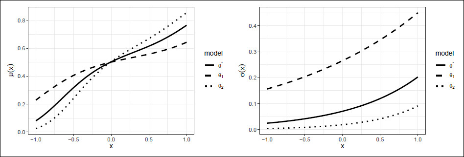
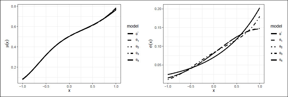
To illustrate the results, we selected two models θ₁ and θ₂ resulting from the perturbed parameters. Table 1 displays the model parameters, optimal design and D_def for the assumed true model θ^* and θ₁ and θ₂. Figure 4 displays their corresponding μ and σ curves.

As can be seen in Figure 4, the model functions for θ₁ and θ₂ look quite different from those for θ^*. Looking at Table 1, we observe that the optimal designs roughly take the same form. For θ₂, the lowest design point x = −0.94 is moved slightly to the right, presumably because the response was not informative enough at x = −1. The D-deficiency for θ₂ is also higher than that for θ₁, but still low. Out of all the 729 models considered, θ₂ was the model with maximum D-deficiency, with most D-deficiencies being close to one.

Figure 4 Model functions for μ and σ for the BB regression models for θ^*, θ₁ and θ₂.

Table 2 Model parameters and optimal designs for the selected model θ^* and four alternative models θ₁ to θ₄.

Model θ	Model parameters	BIC	Optimal design ξ_θ
θ*	α = (0.01, 1.04, −0.63, 0.76) β = (−2.65, 1.06)	6308	$\{\begin{matrix} - 1 & - 0.48 & 0.36 & 1 \\ 0.24 & 0.24 & 0.22 & 0.30 \end{matrix}\}$
θ₁	α = (0.01, 1.01, −0.62, 0.84) β = (−2.51, 1.13, −0.54)	6310	$\{\begin{matrix} - 1 & - 0.50 & 0.31 & 1 \\ 0.24 & 0.21 & 0.27 & 0.28 \end{matrix}\}$
θ₂	α = (0.02, 1.03, −0.73, 0.77, 0.12) β = (−2.65, 1.05)	6315	$\{\begin{matrix} - 1 & - 0.64 & - 0.07 & 0.62 & 1 \\ 0.20 & 0.20 & 0.18 & 0.18 & 0.24 \end{matrix}\}$
θ₃	α = (0.01, 1.02, −0.63, 0.83) β = (−2.49, 0.87, −0.62, 0.52)	6316	$\{\begin{matrix} - 1 & - 0.41 & 0.44 & 1 \\ 0.25 & 0.25 & 0.25 & 0.25 \end{matrix}\}$
θ₄	α = (0.02, 1.00, −0.73, 0.85, 0.15) β = (−2.51, 1.13, −0.54)	6317	$\{\begin{matrix} - 1 & - 0.66 & - 0.04 & 0.59 & 1 \\ 0.20 & 0.18 & 0.21 & 0.18 & 0.23 \end{matrix}\}$

4.2 Sensitivity to model form

The locally optimal designs depend on the prespecified parameter θ not only in model parameters, but also in model form, which we understand to mean the polynomial degrees of μ and σ. To investigate the sensitivity of the optimal designs to the model form, we consider several alternative models to θ^*. In the model selection procedure, these alternative models were relatively comparable to θ^* in terms of the applied model selection criterion, the Bayesian Information Criterion (BIC). Combined, the alternative models and the true model lead to a set of candidate models. Table 2 displays for all candidate models the estimated model parameters, the BIC of the estimated model and the resulting optimal designs for these models. Additionally, Figure 5 displays the corresponding model functions for the candidate models. It can be seen that the form of μ is relatively close, but there are some differences in the estimation of σ.

Figure 5 Model functions for μ and σ for the resulting BB regression models.

Table 3 D-deficiency for all optimal designs.

Design ξ	θ^*	θ₁	θ₂	θ₃	θ₄
ξθ*	1.000	1.015	–	1.041	–
ξθ1	1.013	1.000	–	1.066	–
ξθ2	1.111	1.140	1.000	1.153	1.009
ξθ3	1.020	1.036	–	1.000	–
ξθ4	1.119	1.125	1.008	1.155	1.000
ξ_U	1.650	1.873	1.622	2.093	1.758

To investigate the sensitivity of these designs to model form, we again look a their D-deficiency. For each candidate model in turn, we assume it is the true model and compute the D-deficiencies of the optimal designs resulting from the competing models relative to the optimal designs of the true model. For comparison, we also investigate the performance of a uniform design ξ_U. The resulting D-deficiencies are given in Table 3. Some entries in Table 3 are empty because the designs were singular for the true model. For example, the true model θ₃ cannot be estimated from the design ξ^*, because four design points are insufficient to estimate the fourth-degree polynomial for μ.

As can be seen in Table 3, the optimal designs were relatively robust against the choice of model, with a maximal D-deficiency of 1.155. The D-deficiencies seem to be most affected by the largest polynomial degree in the BB regression model. Assuming a larger polynomial degree for μ adds an extra design point to the design, which is inefficient when the true polynomial degree is lower. Note that the D-deficiency of the uniform design is rather high (ranging from 1.650 to 2.093).

4.3 Sensitivity to optimality criterion

D-optimal designs minimize the generalized variance in the regression parameters. However, to be of practical interest in psychological test norming, the designs should perform well in terms of the variance of the normed score estimates. To investigate the performance of D-optimal designs with respect to normed score estimation, we performed a simulation study. The performance of the D-optimal designs was compared to a standard uniform design.

Figure 6 Sampling variances of *z_kl*-scores for the D-optimal and uniform design, including 95% confidence bands.

Taking θ^* as the true model, we simulated samples from both the D-optimal design and a uniform design. For each sample, we fitted a BB regression model with a third-degree polynomial for μ and a linear relation for σ, that is, the true model. From the fitted models, we estimated for several age values x_l = −1, −0.9, …, 1 and test scores y_k = 0, 1, …, 36 the percentile p_kl and converted this to a commonly used normed score, the z-score z_kl. In total, we simulated 5 000 samples. The simulation results were analysed using the simhelpers package in R (Joshi and Pustejovsky, 2022).

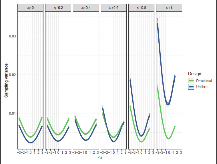
Figure 6 displays the resulting sampling variance of the z-scores for a few selected age values x_l. Because the sampling variances were relatively symmetrical over the design region

X

, only the positive values of x_l are displayed. Figure 6 includes 95% confidence bands based on the Monte Carlo standard error. Following convention in psychological test norming, only z-scores between −3 and 3 are displayed, as more extreme scores can generally not be estimated reliably. Due to floor and ceiling effects for the outer x-values, some z-scores are missing.

From Figure 6, we observe that for more central x-values, the uniform design has lower sampling variance for all z-scores, thus outperforming the D-optimal design. However, both designs have reasonably low absolute sampling variance in the central x-values, especially when compared to the outer x-values. For the outer x-values (e.g., x_l = 0.8, 1.0) the D-optimal design clearly has lower sampling variance. At x_l = 0.6 we observe that the D-optimal design has lower variance in the extreme z-scores only. All in all, this suggests that the uniform design performs somewhat better than the D-optimal design in the centre of the design region and for moderate z-scores and the D-optimal design performs substantially better near the edges of the design region and for extreme z-scores.

5 Discussion

The aim of this article was to derive and characterize D-optimal designs for the BB regression model, motivated by its use in psychological test norming. In doing so, we extend the literature on optimal designs in psychological test norming (Innocenti et al., 2023) to a non-normal and heteroscedastic test score model. Furthermore, we extend the research of Arnoldsson (2003) into D-optimal designs for the BB logistic model. By additionally modelling the dispersion as a function of covariates, we add to research into optimal designs for GAMLSS models (see Atkinson et al., 2014).

The main result of this article is the derivation of D-optimal designs for the BB regression model. In principle, our approach is generalizable to other GAMLSS models and other convex optimality criteria, but the convergence of the numerical procedure should be checked carefully. In general, the D-optimal designs balance mean and dispersion estimation by placing design points at both points of low and high dispersion. Additionally, we present D-optimal designs for the BB logistic regression model in the psychological test norming context. In this context, the binomial denominator in the BB logistic regression model is considerably higher than for the medical context in Arnoldsson (2003), which leads to addition of an internal support point to the D-optimal designs.

Two limitations still impede the practical implementation of the D-optimal designs in psychological test norming. First, the D-optimality criterion is not tailored to normed score estimation and second, the D-optimal designs we derived are only locally optimal. Both limitations are considered in a practical example relevant to psychological test norming. For this practical example, we found that the D-optimal design was relatively suitable for norm estimation. Compared to a uniform design, the D-optimal design substantially reduced the sampling variance of the normed scores at the edges of the design region, while still showing acceptably low sampling variance at the centre of the design region. Second, we found that the D-optimal design was relatively robust to changes in initial model parameters and model form and the quality of the resulting alternative designs was close to the original D-optimal design. In our example, the two limitations are thus of limited effect and the D-optimal designs could be safely applied. Yet, as it is unknown to what extent this can be generalized to other applications, it would be good to resolve the limitations.

The first limitation is the issue of the suitability of D-optimality as a criterion for norm estimation. A possible downside to using D-optimal designs is that they are designed for model parameter estimation and in a sense, weigh all model parameters equally. Consequently, D-optimal designs for BB regression models where the number of model parameters for the mean is larger than for the dispersion, will put less emphasis on the dispersion estimation. However, proper dispersion estimates play a large role in the estimation of extreme norm scores. For the estimation of extreme normed scores, a criterion that puts more weight on the dispersion parameters might be suitable, as is also suggested in Arnoldsson (2003) and Atkinson and Cook (1995). In addition, an optimality criterion that directly minimizes the sampling variance of a normed score of interest could be considered. However, it should be considered that minimizing the sampling variance can be done in multiple ways, for example by minimizing maximum sampling variance over the design region, the integrated variance or a combination of the two (see Walsh et al., 2024). Which criterion is best suited for the psychological test norming context remains to be investigated.

The second limitation concerns the sensitivity of the D-optimal designs to the initial model parameters. This limitation could be addressed by extending the locally optimal designs to globally optimal designs, for example, with a Bayesian, maximin or adaptive strategy (see e.g., Atkinson and Woods, 2015). Prior information on the test score model could be based on previous test versions or similar tests in other countries (see also Voncken et al., 2021).

Further ideas for future research include adding extra predictors to the BB regression model, for example, categorical variables representing gender or educational level, as is common in neuropsychological testing (e.g., Zec et al., 2007; Keefe et al., 2008); extending the model to allow for simultaneous responses, accounting for administration of several subtests at once; incorporating a nested structure in the model, for samples which are collected from pupils within schools (see e.g., Moerbeek et al., 2000). Last, we assumed in this study that age is a fully controllable variable. This assumption could also be addressed in further research.

This study adds to the optimal design literature and advances its application in psychological test norming. Even though the practical relevance of the resulting D-optimal designs should be studied in further research, this study makes a valuable step towards integrating the efficiency of optimal design theory with the current practice in psychological test norming.

Acknowledgements

We want to thank the publisher BSL Media and Learning of the Schlichting-3 test for providing their empirical data. We also thank the anonymous reviewers for their valuable and constructive comments, which helped improve the manuscript.

Declaration of Conflicting Interests

The authors declared no potential conflicts of interest with respect to the research, authorship and/or publication of this article.

Funding

The authors disclosed receipt of the following financial support for the research, authorship and/or publication of this article: This research was funded by the Dutch Research Council NWO, under grant number 406.27.GO.022.

ORCID iDs

Klazien de Vries https://orcid.org/0009-0007-9302-1562

Marieke E. Timmerman https://orcid.org/0000-0003-1579-6964

Casper J. Albers https://orcid.org/0000-0002-9213-6743

References

Arnoldsson G (2003) Optimal designs for beta-binomial logistic regression models. Journal of Applied Statistics, 30, 939–51. doi: 10.1080/0266476032000076001.