The Romano–Wolf multiple-hypothesis correction in Stata

Consider inference for a generic parameter θ. In what follows, we will refer to data used to estimate this parameter as X and the value estimated using these data as $\widehat{\theta }$. When a single null hypothesis H about θ is tested against a single alternative hypothesis H′, a decision rule can be defined based on the rate of a type I error, defined as

The test could be a two-sided test, such as H : θ = θ ⁰ versus H′ : θ ≠ θ ⁰, or it could be a one-sided test, such as H : θ ≤ θ ⁰ versus H′ : θ > θ ⁰. The quantity θ ⁰ refers to the null value of interest defined by the researcher and is often θ ⁰ = 0.³ The type I error is defined when the null hypothesis is true, and as such, Pr_θ0 refers to the probability of (falsely) rejecting the null when θ ⁰ is the actual value of the parameter. If the probability in (1) is bounded above by a value α, then α is the significance level at the test. Often, a particular value of α is chosen in advance, such as α = 0.05, and the testing procedure is designed to meet this criterion. Alternatively, to avoid somewhat arbitrary criteria, one can report a p-value, here p, that fulfills (at least asymptotically)

for every 0 ≤ α ≤ 1 and is defined as the smallest value of α at which H would be rejected. Smaller values of p provide more evidence in favor of the alternative hypothesis H′.

The validity of this error rate of α assumes that a single null hypothesis is tested. We now extend the setting to a family of S null hypotheses ${\left\{H_s\right\}}_{s=1}^S$, which are related to parameters ${\left\{{\theta }_s\right\}}_{s=1}^S$, versus respective alternative hypotheses ${\left\{H_s^{\prime }\right\}}_{s=1}^S$. If the error rate in (1) is only controlled at α one null hypothesis at a time, it is clear that the probability of committing at least one type I error across the S null hypotheses will generally exceed α.⁴ Following Lehmann and Romano (2005b), we let I ⊆ {1,…, S} denote the set of true null hypotheses, and the FWER is then defined as

To account for multiple-hypothesis testing, we seek to control the FWER at level α. By definition, if all the null hypotheses are false, the FWER is equal to 0.

A traditional solution has been to implement the Bonferroni procedure, which consists of rejecting any H_s for which the corresponding p-value, p_s, satisfies p_s ≤ α/S. This procedure provides strong control⁵ of the FWER (see, for example, Lehmann and Romano [2005a, 350]); however, it often has low power to detect false null hypotheses, particularly when the number of hypotheses is large. A procedure that has greater power, while still maintaining control of the FWER was described in Holm (1979). This is a stepdown procedure that begins by ordering the individual p-values such that p _{( 1 )} ≤ p _{( 2 )} ≤ · · · ≤ p _{( S )}, corresponding to hypotheses H _{( 1 )} , H _{( 2 )} ,…, H _{( S )}; in this way, the hypotheses are ordered according to their significance. H _{( 1 )} is rejected if and only if (iff) p _{( 1 )} ≤ α/S, just as would be the case for Bonferroni. But if it is rejected, then H _{( 2 )} is rejected if p _{( 2 )} ≤ α/(S − 1), which is a more lenient criterion. The procedure proceeds in this manner until at some step s, p _{( s )} > α/(S −s+1), and then it stops. (If the stopping criterion is never met, the procedure rejects all S hypotheses.) The Holm procedure rejects all hypotheses rejected by the Bonferroni procedure but potentially also rejects other hypotheses.

Both the Bonferroni and the Holm procedures are easy to implement and only require the list of individual p-values ${\left\{p_s\right\}}_{s=1}^S$. But this convenience comes at a (potentially) severe loss in power. The two procedures achieve control of the FWER by assuming a worst-case dependence structure among the p-values, which is close to the individual p-values being independent of each other. If the FWER is controlled in the worst case, it is always controlled. But if there is noticeable dependence among the p-values, it would be possible to maintain control of the FWER while increasing power at the same time.

We now illustrate this point with a simple example. Let’s say there are S = 100 hypotheses under test, and one wants to control the FWER at level α = 0.05. The p-values p_s are based on test statistics T_s that have a joint normal distribution with common variance 1 and common pairwise correlation ρ. The mean of all test statistics T_s for which H_s is true is equal to 0. The tests are one-sided in the sense that

where Z ∼ N(0, 1) and t_s is the observed realization of T_s. We consider the following single-step procedure: Reject H_s iff p_s ≤ c_ρ, where c_ρ is a common cutoff allowed to depend on ρ. The Bonferroni procedure uses c_ρ ..= 0.05/100 = 0.0005, irrespective of ρ. But as a function of ρ, the following, less conservative, cutoffs suffice to guarantee control of the FWER:

(Apart from ρ = 0 and ρ = 1, the cutoffs c_ρ need to be determined by numerical simulations and are, therefore, subject to some small simulation error.) In particular, when ρ = 1, all p-values are perfectly correlated, meaning that there really is only a single shared hypothesis under test, in which case it is allowed to use the naïve cutoff α = 0.05 itself. In general, the larger is ρ, the larger is the cutoff c_ρ, and thus, the easier it becomes to reject false hypotheses, which increases power. Similar considerations carry over to the more general case when pairwise correlations are not constant and to stepwise procedures.

Hence, as described above, if there exists noticeable dependence among the p-values, it would be possible to maintain control of the FWER while increasing power at the same time. To this end, resampling-based multiple-testing procedures have been proposed in the literature. By resampling from the observed data, one can mimic the true dependence structure of the p-values (or, equivalently, among the test statistics) and thus account for it (in an implicit fashion). An early such proposal goes back to Westfall and Young (1993), who use the bootstrap to account for the dependence structure of the p-values. This procedure (described in Westfall and Young [1993, algorithm 2.8] and summarized in appendix A of this article), assumes a certain subset pivotality condition, which is used in establishing FWER control. Roughly speaking, this condition means the following: Take any nonempty, strict subset of hypotheses (out of all hypotheses under test) and look at the random vector of corresponding test statistics. Then the joint distribution of this random vector is unique in the sense that it does not depend on whether the remaining hypotheses (not under test) are true or false. For a precise definition, see Romano and Wolf (2005b, example 2).

Subset pivotality can be violated in certain applications and is thus undesirable, because in such instances the Westfall–Young procedure only guarantees weak control of the FWER. An example where this condition is violated is given by jointly testing the entries of a correlation matrix. Take the case of independent and identically distributed multivariate observations of dimension three. The multiple-testing problem concerns the three (distinct) pairwise correlations

where ρ_ij denotes the correlation between components i and j of any of the observations. The individual test statistics are the sample correlations, denoted by ${\widehat{\rho }}_{ij}$, and regularity conditions are in place such that the (normalized) vector $\left({\widehat{\rho }}_{12},{\widehat{\rho }}_{13},{\widehat{\rho }}_{23}\right)\prime$ has an asymptotic normal distribution. Now assume that one is only interested in testing the subset {H ₁₂ , H ₁₃}. Then the asymptotic distribution of the vector $\left({\widehat{\rho }}_{12},{\widehat{\rho }}_{13}\right)\prime$ depends on ρ ₂₃, so it depends on whether the remaining hypothesis (not under test) H ₂₃ is true or false; see Romano and Wolf (2005b, example 7) for further details.

Having said this, the procedure of Westfall and Young (1993) is available for Stata, as provided in Reif (2017), with additional discussion in Jones, Molitor, and Reif (2019).

More recently, the Romano–Wolf multiple-hypothesis correction has been proposed, as described in Romano and Wolf (2005a,b) as well as in the subsection below. This procedure also uses resampling and stepdown procedures to gain additional power by accounting for the underlying dependence structure of the test statistics. However, and crucially, this procedure does not require the subset pivotality condition and is thus more broadly applicable than the Westfall–Young procedure.

Romano and Wolf (2005b) propose a procedure that controls the FWER at a given level α; hence, this procedure leads to a decision to reject or not reject for each null hypothesis H_s considered, for s = 1,…, S. In follow-up work, Romano and Wolf (2016) describe how to compute p-values adjusted for multiple testing, which is a more flexible approach. Having adjusted p-values, one immediately knows which hypotheses to reject for any level α, as opposed to just for a specific level α. In other words, if one were to consider a different level α compared with a prior analysis, one would have to rerun the procedure of Romano and Wolf (2005b) with the new value of α; on the other hand, having adjusted p-values at hand, no new analysis is needed. The rwolf command returns the p-value adjustment documented in Romano and Wolf (2016), following Romano and Wolf’s (2005b) Studentized StepM Procedure (algorithms 4.1–4.2). Here we describe the algorithms implemented, before turning to the precise syntax in the following section.

Prior to describing the p-value adjustment algorithm implemented in rwolf, we first describe the Romano and Wolf (2005b) procedure. The algorithm below is based on a bootstrap procedure; by default, rwolf is based on the standard Efron (1979) bootstrap (see Romano and Wolf [2005b, appendix B] for discussion). In section 4, we discuss extensions to alternative bootstrap methods, such as the block bootstrap.⁶

As above, suppose we wish to test S hypotheses, using data X. Each hypothesis H_s is associated with a parameter of interest θ_s, an estimator of this parameter ${\widehat{\theta }}_s$, and a corresponding standard error ${\widehat{\sigma }}_s$ ⁷ For notational convenience, we generally assume that ${\theta }_s^0=0$, for s = 1,…, S. We assume further that the alternative hypotheses are either all one-sided of the type $H_s^{\prime }:{\theta }_s>0$ or all two-sided of the type $H_s^{\prime }:{\theta }_s\ne 0$.⁸ A Studentized test statistic for H_s is given by⁹

Next consider M resampled data matrices of X, denoted by $X_{ }^{*},\dots ,X_M^{*}$. They give rise to estimators, denoted by ${\widehat{\theta }}_s^{*,m}$, and corresponding standard errors, denoted by ${\widehat{\sigma }}_s^{*,m}$, for m = 1,…, M. For each resample m and for each hypothesis H_s, a Studentized null statistic is given by

These statistics $t_s^{*,m}$ are centered around 0 given that the numerator consists of a resample estimate minus the original estimate (rather than the null parameter), and as such, the distributions of $t_s^{*,m}$ will form the null distributions for the procedure.¹⁰

In case the alternative hypotheses are two-sided of the type $H_s^{\prime }:{\theta }_s\ne 0$, it is important to work with the absolute values of the test statistics. To keep the notation uniform in the algorithm outlined below, in slight abuse of notation, we will use the following convention in the two-sided case (but not in the one-sided case):

Finally, as above, we will relabel hypotheses in order of significance—but now based on their test statistics t_s instead of their p-values p_s, as was done before by the Holm procedure—such that H _{( 1 )} refers to the hypothesis with the largest corresponding test statistic [labeled t _{( 1 )}], and H _{( S )} refers to that with the smallest [labeled t _{( S )}]. In what follows, we denote by ${\max }_{t,j}^{*,m}$ the largest value of the vector $\left\{t_{\left(j\right)}^{*,m},\dots t_{\left(s\right)}^{*,m}\right\}$:

For a given j, we denote by $\widehat{c}\left(1-\alpha ,j\right)$ the empirical 1 − α quantile of the statistics ${\left\{{\max }_{t,j}^{*,m}\right\}}_{m=1}^M$. For example, in a case where one is testing S = 4 hypotheses, ${\max }_{t,1}^{*,m}$

denotes the maximum value of $\left\{t_{\left(1\right)}^{*},t_{\left(2\right)}^{*},t_{\left(3\right)}^{*},t_{\left(4\right)}^{*}\right\},{\max }_{t,2}^{*,m}$ denotes the maximum value of the subvector $\left\{t_{\left(2\right)}^{*},t_{\left(3\right)}^{*},t_{\left(4\right)}^{*}\right\}$ (that is, the vector of test statistics corresponding to the three least significant hypotheses only), and so on. At last, we simply have $\max t_{\left(4\right)}^{*,m}=t_{\left(4\right)}^{*,m}$. An important consequence is that $\widehat{c}\left(1-\alpha ,j\right)$ is weakly decreasing in j; that is, $\widehat{c}\left(1-\alpha ,j\right)\ge \widehat{c}\left(1-\alpha ,j+1\right)$, for j = 1,…, S − 1.

Based on the above, the principal stepdown multiple-testing procedure at level α (based on algorithm 3.1 from Romano and Wolf [2016]) can be summarized as follows.

As was the case with the procedure of Holm (1979), this correction is a stepdown procedure: ĉ(1 − α, j) is weakly decreasing in j and, as such, the criterion for rejection is more demanding for more significant hypotheses and becomes less demanding for less significant hypotheses. Given that the null distributions based on ${\max }_{t,j}^{*,m}$ are based on resamples of the original data, they implicitly account for the underlying dependence structure of the test statistics, leading to potentially considerable gains in power over the Holm procedure, which assumes a worst-case dependence structure.

The above algorithm leads to a decision whether to reject or not reject for each null hypothesis H_s at a given significance level α. However, additionally and perhaps more conveniently, a multiple-testing-adjusted p-value can be directly computed for each H_s, as described in the algorithm below. This algorithm is a generalization of a resample-based p-value for a single null hypothesis, which can be defined as (Romano and Wolf 2016; Davison and Hinkley 1997, 158).

Note that other definitions exist.¹¹ To generalize this to a situation where multiple hypotheses are considered, rwolf implements the following algorithm to compute the p-values using the distribution of ${\max }_{t,j}^{*,m}$, following Romano and Wolf (2016, algorithm 4.2).

Either option can be implemented in the rwolf command, as described in section 3.

rwolf is an e-class program and returns many elements in the e() list. It returns scalars corresponding to each calculated Romano–Wolf p-value, which are available as e(rw_ depvar ), where depvar refers to the name of each dependent variable. If multiple independent variables are considered, a scalar for each p-value corresponding to each independent–dependent variable pair will be returned as e(rw_ depvar_indepvar ). A matrix is also returned as e(RW) providing the full set of Romano–Wolf-corrected p-values. If the holm option is indicated, p-values according to Holm (1979) will be returned in column 4 of this matrix. Again if multiple independent variables are considered, a matrix named e(RW_ indepvar ) will be returned corresponding to each depvar.

We begin by presenting a particularly simple case. Consider the following linear model, in which 10 outcome variables y^s are regressed on a single independent variable, treat. Superscript-s terms refer to each of the multiple outcomes, of which there are a total of S, or their determinants. The data-generating process (DGP) is simulated as

for observation i. For each observation i, the 10 stochastic error terms ${\epsilon }_i^s$ are drawn from a multivariate normal (mvn) distribution, following

with ρ ≥ 0, and the independent variable of interest, treat _i, is generated as treat _i $1_{\left\{U_i>0.5\right\}}$, where 1 denotes the indicator function and U_i ∼ U(0, 1). This is a highly stylized setting, but it allows us to vary the correlation between the multiple outcome variables of interest (y ¹ , y ² ,…, y ¹⁰) via the parameter ρ, as well as the impact of treatment via the parameter ${\beta }_1^s$. In particular, we can examine both the empirical fwer and the empirical proportion of false null hypotheses that get rejected (that is, power). We can examine this performance not only for the Romano–Wolf procedure but also for Holm’s procedure and for naïve procedures that do not account for multiple testing.

We consider a series of simulations based on N = 100 observations. Each null hypothesis is that ${\beta }_1^s=0$, versus the two-sided alternative hypothesis ${\beta }_1^s\ne 0$. Across simulations, we vary the number of models in k = 1, 2,…, 10 for which ${\beta }_1^s=0$, as well as ρ, the correlation between outcomes induced by the stochastic error terms. Below, we document one such simulation and resulting multiple-hypothesis correction.

In the simulation below, each of the 10 ${\beta }_1^s$ terms is equal to 0, and the correlation between draws in the mvn distribution is set at ρ = 0.25. We follow the dgp described above, where first we simulate treat _i (as treat), and then we generate ε_i as a draw from an MVN. This draw is generated using a transformation of independent normal draws using a Cholesky decomposition of the desired covariance matrix and Stata’s matrix score command to multiply row vectors.¹²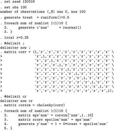

Once we have simulated the N × S matrix Y in the above code, we apply the Romano–Wolf stepdown correction. Here we are considering the S = 10 outcome variables y1–y10 and the single independent variable treat. We request that the command perform 1,000 bootstrap repetitions, which, given the lack of other options, will be performed by resampling observational units with replacement. By specifying the nodots and holm options, we request that no dots be displayed on the Stata output to indicate the degree to which the resample procedure has advanced, and we request for rwolf to return p-values corrected using Holm’s (1979) procedure (which will be listed in the final column of tabular output and saved in the returned e() list).

The command returns a list of p-values associated with each of the multiple outcomes. The column Model p-value lists the analytical p-values coming directly from the estimated regression model based, in each case, on the t statistic and the (inverse) cumulative distribution function of a t distribution with appropriate degrees of freedom. The column Resample p-value lists the resampling-based p-values as per (6), which also do not correct for multiple testing. In the case of both of these uncorrected procedures, despite the fact that all true β ₁ values were 0, many of the hypotheses that β ₁ = 0 are rejected at α = 0.05. In particular, the variables y4 and y7 have p-values below 0.05 for both uncorrected procedures. The third column displays the Romano–Wolf adjusted p-values, where we note that now no null hypothesis is rejected (even at α = 0.10).

The simulated example above provides one example of a multiple-hypothesis correction based upon a known DGP. To examine the performance of the rwolf command (and the Romano–Wolf correction in this context) more generally, we can examine the error rates and proportion of hypotheses correctly rejected when we vary the number of values of β ₁ ^s = 0 and the correlation between outcomes, ρ. We consider such an example in tables 1 and 2 (which are in the spirit of tables 1–3 in Romano and Wolf [2005a]). The first table considers the proportion of times at least one null hypothesis is rejected when the null hypothesis is actually true (the FWER), and the second table considers the proportion of hypotheses that are correctly rejected when the null hypothesis is false (the power of the tests).¹³

In these tables, we consider 1) a series of models where all of the β ₁ ^s terms are equal to 0 (presented in panel A of table 1), 2) a series where half of the β ₁ ^s terms are equal to 0 and the other half are equal to 0.5 (presented in panel B of table 1 when considering FWERs and panel A of table 2 when considering power),¹⁴ and 3) a series where all of the β ₁ ^s terms are equal to 0.5 (presented in panel B of table 2). Case 1 is not considered in table 2 given that all null hypotheses are true and so cannot be “correctly rejected”. Similarly, case 3 is not considered in table 1 given that all null hypotheses are false and so the FWER is trivially equal to 0 given that they cannot be “incorrectly rejected”. Across columns, we vary the degree of correlation between outcomes, from ρ = 0 in the first two columns, to ρ = 0.75 in the final two columns. The nominal levels for the FWER are set at α = 0.05 and α = 0.10, respectively.

Here we briefly discuss the performance of the rwolf command and note several important features of the Romano–Wolf multiple-hypothesis correction. In particular, we always present the performance criteria for three testing procedures: those corresponding to the naïve case, where no correction for multiple-hypothesis testing is made; those corresponding to Holm’s procedure; and those corresponding to the Romano–Wolf procedure.

In panel A of table 1 (where all values for ${\beta }_1^s=0$), it is clear in the uncorrected case that the empirical FWERs greatly exceed nominal levels of α = 0.05 and 0.10. When all outcomes are uncorrelated, these values are 0.396 and 0.642, respectively, suggesting a large proportion of families in which a null hypothesis is incorrectly rejected, in line with that predicted in theory.¹⁵ As the correlation between outcomes grows, these naïve values fall closer to the nominal levels but still considerably exceed desired error rates.

With the Holm correction, we observe that the FWER is controlled at both the 5% and 10% levels. This is observed regardless of the degree of correlation considered, between ρ = 0 and ρ = 0.75. Similar control is observed with the Romano–Wolf procedure. Indeed, in each case the empirical FWER is very close to the desired nominal rate of 0.05 or 0.10, respectively. In panel B of table 1 (where 5 of the 10 hypotheses should not be rejected), we again observe that the FWER without multiple-hypothesis correction still substantially exceeds desired error rates but is successfully controlled at no more than α with both the Holm and Romano–Wolf procedures.

In table 2, we can examine the relative power of the Holm and Romano–Wolf procedures for rejecting false null hypotheses. In panel A of table 2, we return to the case considered in panel B of table 1, here considering the power of the tests instead. In this setting, the naïve case of no multiple-hypothesis correction allows us to reject a large proportion of false null hypotheses (at the cost of the FWER documented in table 1).

In the case of Holm and Romano–Wolf, we observe relatively similar rates of correct rejection when the correlation between outcomes is 0, but as expected, as the correlation between outcomes grows, the Romano–Wolf procedure substantially improves relative to Holm’s procedure. For example, in the final column of panel A, we reject 59.4% of false null hypotheses using the Romano–Wolf procedure versus only 46.8% using Holm’s procedure, a 27% improvement in rejection rate. A similar pattern is observed in table 2, panel B (where all null hypotheses are false). Initially, when the correlation between outcomes is 0, Holm’s and Romano–Wolf’s procedures have similar power; however, to the degree that ρ increases, the Romano–Wolf procedure becomes relatively more powerful.

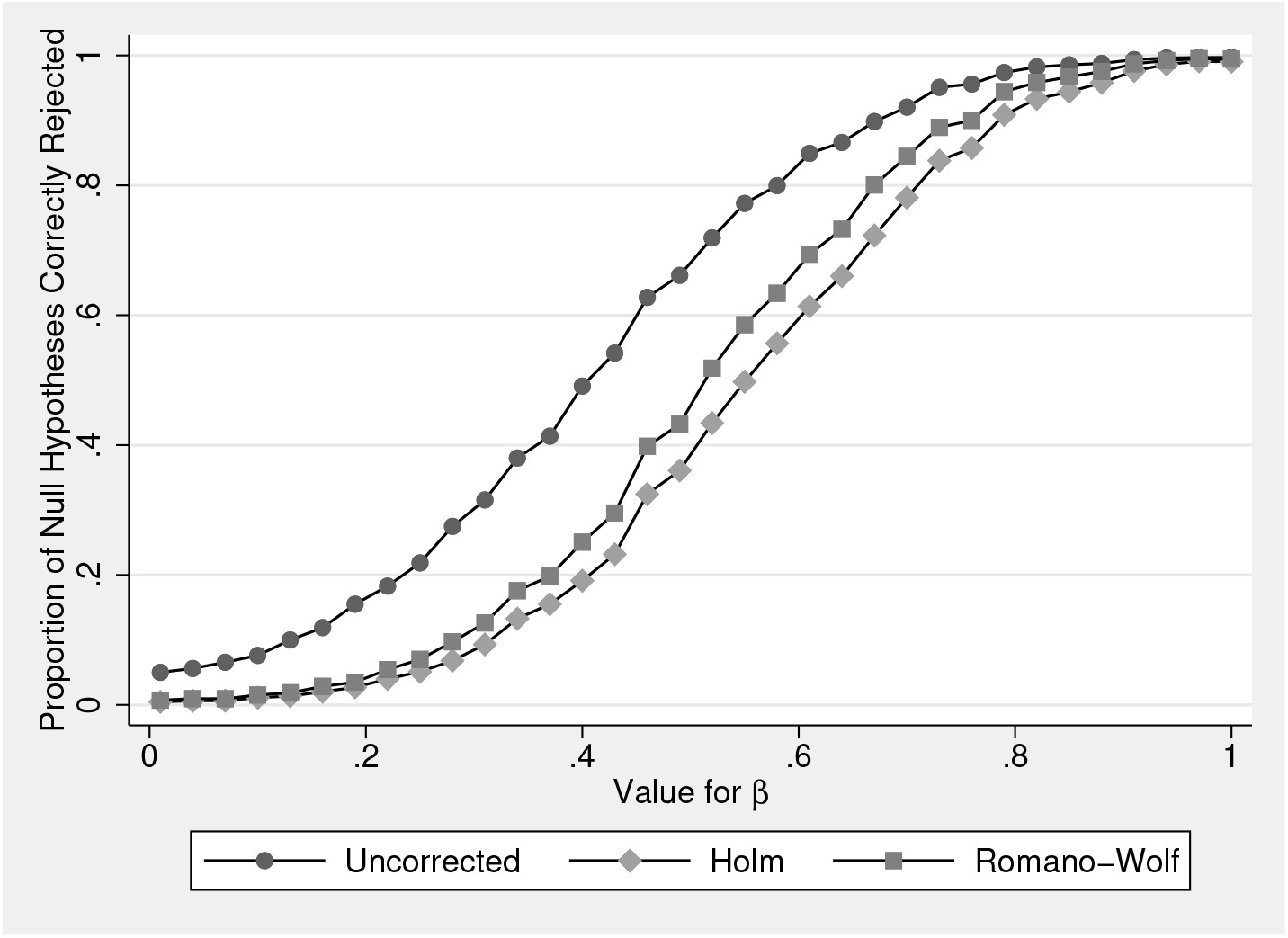
In table 2, we consider the relative power of testing procedures for rejecting false null hypotheses with a particular value for β ₁ ^s, in this case, ${\beta }_1^s=0.5$ for all cases where ${\beta }_1^s\ne 0$. The relative power of these procedures will depend on the actual value of β ₁ ^s. Below, in figure 1, we consider how these rates of rejection vary with ${\beta }_1^s$ values. In the figure, we consider the case corresponding to table 2 panel B (where all ${\beta }_1^s\ne 0$) and where ρ = 0.5. We present values of ${\beta }_1^s$ varying from 0.01 to 1, in steps of 0.03. All other details follow the DGP in (8).

For each value of β ₁, we run 1,000 simulations, in each case calculating the unadjusted p-values, and the Holm and Romano–Wolf p-values using the rwolf command. Across the 1,000 simulations, we examine the proportion of null hypotheses correctly rejected. As expected, the power when not conducting any multiple-hypothesis correction is greatest (at the cost of exceeding the FWER if the null hypothesis were true). To the degree that the correlation between outcomes approaches ρ = 1, the power of the Romano–Wolf procedure will approach the power of the procedure with no multiplehypothesis correction.

Of interest is the relative performance of Romano–Wolf’s versus Holm’s correction. Here, given that ρ = 0.5, the power of the Romano–Wolf correction dominates the power of the Holm correction across each value for β ₁. This difference is particularly notable at values of β ₁ between 0.4 and 0.6, and all disappear as β ₁ becomes large, implying sufficient power to reject all null hypotheses regardless of the correction procedure. When β ₁ = 1, each of the procedures results in rejection rates of around 100%.

The simulated examples based on rwolf displayed previously provide a standard implementation where multiple outcome variables are regressed on a single independent (treatment) variable, each using an ordinary least-squares regression. However, the standard command syntax of rwolf allows for many extensions of this baseline implementation. This includes the use of alternative estimation methods (for example, IV regression, probit, and other Stata estimation commands), the implementation of one-sided tests, or the use of alternative bootstrap routines (for example, block and stratified bootstraps). To document several such extensions, we turn to an alternative example below, modeled after a simple IV regression example based on system data, as described in the help file of Stata’s ivregress. Here we extend to a case with multiple outcomes and examine both a one- and a two-sided test.

We begin with a (default) two-sided test, where we follow the implementation of the two-stage least-squares estimate from the ivregress help file.¹⁶ We use the same specification, where along with the outcome variable rent, we also consider three other variables: popden, popgrow and hsng. We do not make any claim to causality or consistency of the resulting estimates. These are simply shown as an illustration of the rwolf command with an IV regression. In each case, the independent variable of interest is hsngval, and this is instrumented with the variables indicated in the iv() option. We include pcturban as an additional control. We use 10,000 bootstrap replications (bootstrapping on observational units) and request a graph of the null distributions used in testing be reported (as discussed below).

The setup and output of this Romano–Wolf correction is displayed below. In this example, the p-values from the original IV models are quite low, suggesting evidence against the null that each coefficient on the variable hsngval is 0. The Romano–Wolf correction displayed in the final column results in inflated p-values (as designed), though the adjusted p-values are still relatively low.

Below, we document the same procedure but here conducting one-sided hypothesis tests. In each case, the null hypothesis in these tests will be of the form H ₀ : β ₁ ≤ 0, versus the alternative H ₁ : β ₁ > 0, where β ₁ is the coefficient on hsngval in the second stage of the IV regression. For the sake of illustration, we multiply the two outcomes by −1, such that the sign on ${\widehat{\beta }}_1$ estimated in each IV regression is greater than 0. Along with the syntax described previously, the implementation of one-sided tests requires the use of the option onesided(). If onesided(negative) is specified, the null will be H ₀ : β ₁ ≤ 0; that is, negative values will provide more support for the null. On the other hand, if onesided(positive) is specified, the null will be H ₀ : β ₁ ≥ 0 in each case, such that positive values will provide more support for the null.

In each example, we specified the graph option to request as output the null distributions used to calculate the p-value in each case. Examining these distributions allows us to empirically observe how much more demanding the Romano–Wolf correction is compared with an uncorrected test.

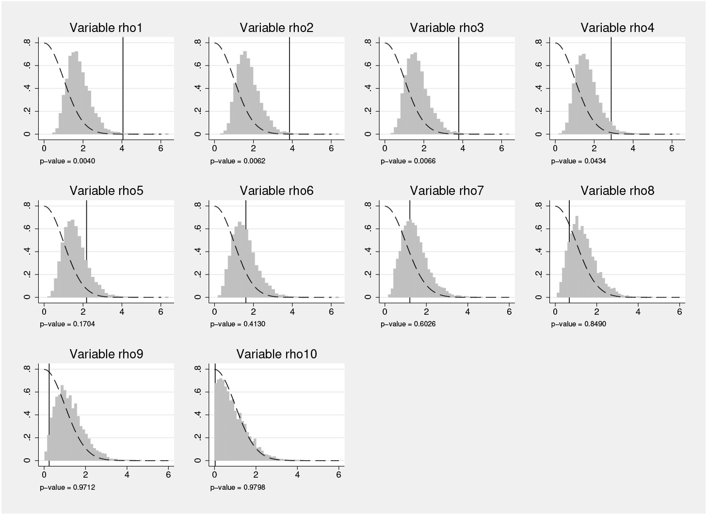
In figure 2 panel (a), we display these distributions in the two-sided case. Here the histogram presents the absolute value of each (Studentized) estimate from the bootstrap replications where the null is imposed, and the black dotted line presents an exact half-normal distribution. The actual Studentized value of the regression coefficient is displayed as a solid vertical line. In the top left panel, the first null distribution is considerably more demanding than the theoretical distribution, given that it accumulates the maximum coefficient estimated across each outcome. These null distributions become increasingly less demanding in the top right and bottom left panels because previously tested variables are removed from the pool to form the null distributions. Finally, in the bottom right corner (for the least significant variable), the null distribution is based on bootstrap replications from only this variable, and as such, the null distribution closely approximates the theoretical half-normal distribution.

In figure 2 panel (b), we present the same null distributions but now based on the one-sided tests. Here the histogram documents the maximum values across the multiple variables in each bootstrap replication, and the black dotted line presents the theoretical normal distribution. Once again, when we consider outcomes for which more significant relationships are observed, the empirical distribution used to calculate the corrected p-value is considerably more demanding than the black dotted distribution, which would be used under no correction and a normality assumption. In the case of the least significant variable (popden), these two distributions are similar given that the null distribution is based only on Studentized regression estimates of the single regression where this is the outcome variable.

Each previous example has been based on the simple rwolf command syntax where a single independent variable is regressed on multiple outcome variables. This is frequently sufficient for a large number of implementations, such as cases where a single experimental treatment is assigned, and various outcomes are measured. In this case, the rwolf command can be implemented in one line and takes care of everything, including the full process of bootstrap draws, estimation of regression coefficients and standard errors, as well as the generation of null distributions and p-values. However, Romano–Wolf p-values can also be calculated for more complex setups, if the user wishes to pass the command the already-bootstrapped (or permuted) statistics and standard errors that have been calculated from the underlying models of interest. We document this flexibility in what remains of this section, using a bootstrap approach where our statistics of interest are a series of correlations.

We use an example and data documented in Westfall and Young (1993), which was also previously used to demonstrate the effectiveness of the Romano–Wolf procedure in Romano and Wolf (2005a). Although we refer to this as a nonstandard example, it is only nonstandard in the way it interacts with the syntax of rwolf, given that the multiple tests are based on several independent variables and as such do not allow for a single independent variable to be indicated using the indepvar() option.

This example considers pairwise correlations between state-average standardized Scholastic Aptitude Test (SAT) scores and several other state-level measures for the 48 mainland U.S. states plus Hawaii. These data—consisting simply of state-level measures of several variables of interest—are provided in table 6.4 of Westfall and Young (1993, 197) as well as in the replication materials for this article. The variables considered are satdev (the residuals from a regression of state-level SAT scores on the square root of the percent of students taking the exam in a given state), the student/teacher ratio in the state, the teacher salary, the percent of the population that is black, and the crime rate of each state.

In this case, the statistics of interest refer to simple correlations between pairs of variables of interest, and p-values will be corrected for the fact that we are testing 10 hypotheses. To construct null distributions following (4) and (5), the rwolf command requires an estimate of the original parameter of interest in each case (the pairwise correlation) along with a standard error. These values are used to construct t_s (as defined in section 2.2) for each of the s multiple hypotheses and to order the hypotheses in terms of their relative significance. The command additionally requires the results from M bootstrap replicates, where a resampled estimate of each statistic and its standard error is provided. 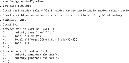We document such a case below, where in each of the multiple hypotheses the parameter of interest is the correlation between variables ρ (which can be simply calculated using corr in Stata) and its standard error, which, assuming normality, is calculated as (Bowley 1928; Zar 2010)¹⁷

To generate the various components that rwolf uses to implement the multiplehypothesis correction, we first open the data and define in locals var1 and var2 the corresponding pairs to be tested. The idea in these locals is that we wish to calculate the correlation between the first variable listed in var1 and the first variable listed in var2, the correlation between the second variable listed in var1 and the second variable listed in var2, and so forth, through the correlation between the last variable listed in var1 and the last variable listed in var2. We calculate these correlations one by one in the foreach loop in the code below. We loop over elements of the local var1, and we take corresponding elements one by one from local var2 using Stata’s tokenize command.¹⁸ These correlations and standard errors from the original data are then saved, respectively, as locals c’i’ and s’i’ to be later passed to the rwolf command. Finally, we generate two series of 10 empty variables, rho1–rho10 and std1–std10, which will later be populated by resample-based correlation estimates and their standard errors.

A bootstrap procedure is then implemented based on 5,000 resamples. We initially expand the dataset to have 5,000 observations to store each of the bootstrap estimates; however, prior to calculating the correlations and standard errors in each replicate, we work only with the 49 state-level observations with SAT data. Each replicate is implemented in the main forvalues loop below. Within each of these 5,000 iterations, we first issue a preserve command to later restore the data toward the end of each iteration; this way, the bootstrap resample (bsample) begins with the original data in each iteration. Within each loop, lines 7–12 calculate the bootstrap correlations and corresponding standard errors, which are then filled in line by line in the variables rho1–rho10 and std1–std10 at the end of each loop.

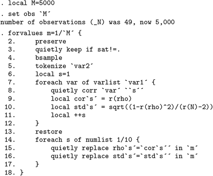
Once we have stored the original estimates plus their standard errors and have variables containing resampled estimates along with their resampled standard errors, we can simply request the multiple-hypothesis correction from rwolf, as laid out in section 3. This is implemented below.

We pass to rwolf the varlist consisting of resampled estimates. The stdests( varlist ) option consists of bootstrap standard errors. Finally, the original correlations and standard errors from the (original) data are passed as numlists in pointestimates() and stderrs(). The graph option requests that a graph be produced documenting the null distributions used in each test, and noplusone requests that the p-value be calculated following (7) rather than the standard (6).

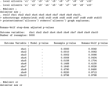
In this nonstandard implementation, no Model p-value is returned because rwolf itself does not estimate the original correlations, simply working with the estimates provided from the above code. In this case, we observe the Resample p-value (which is not corrected for multiple-hypothesis testing), which is the results of comparing each original estimate with the null distribution, and the Romano-Wolf p-value, where the multiple-hypothesis correction has been implemented as indicated in section 2.2. These results are similar to those observed in Romano and Wolf (2005a, table 4) and would result in rejecting the same hypotheses if standard cutoffs (such as α = 0.01, α = 0.05, or α = 0.10) were used.

In figure 3, we present the graph of null distributions, based on (5), for each hypothesis. As implied by the multiple-hypothesis testing algorithm, the null distributions become less demanding while moving from the most significant variable (top left-hand panel) to the least significant variable (left-hand panel in the final row).