

Research and application of XGBoost in imbalanced data
Abstract
Introduction
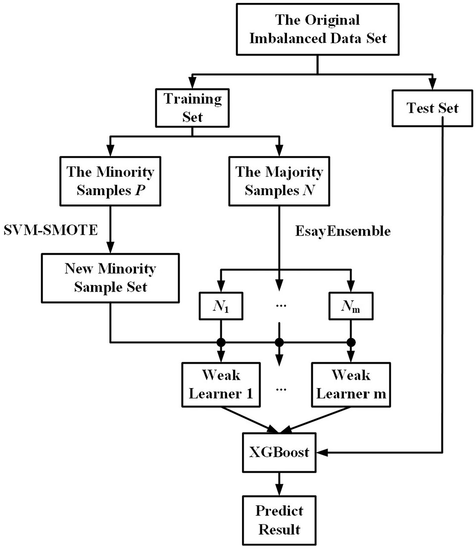
Related algorithms
SVM–SMOTE
EasyEnsemble
| Input: training set , the number of weak learners of AdaBoost , the learning algorithm of AdaBoost |
| 1. Divide the training set to obtain the minority sample set and the majority sample set , , and select subsets from ; |
| 2. For Randomly select subset from so that ; let , train an AdaBoost learner constructed by weak learners on , record the weight of each weak learner and the ensemble decision threshold , that is . End |
| Output: the prediction result of the test sample is |
XGBoost
Algorithm optimization and design
Regularization term optimization
Classification algorithm
Experiment and result analysis
Experimental platform and data introduction
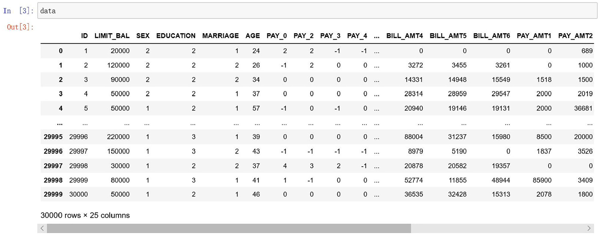
| Number | Features | Description |
|---|---|---|
| 1 | ID | Customer’s unique identification |
| 2 | LIMIT_BAL | Credit line (in NT), including personal and family credit lines |
| 3 | SEX | Customer’s gender (1 = male; 2 = female) |
| 4 | EDUCATION | Customer’s educational level (1 = master’sdegree and above;2 = undergraduate; 3 = high school; 4 = others) |
| 5 | MARRIAGE | Customer’s marital status (1 = married;2 = unmarried; 3 = other) |
| 6 | AGE | Customer’s age |
| 7 | PAY_0 | Repayment status in September |
| 8 | PAY_2 | Repayment status in August |
| 9 | PAY_3 | Repayment status in July |
| 10 | PAY_4 | Repayment status in June |
| 11 | PAY_5 | Repayment status in May |
| 12 | PAY_6 | Repayment status in April |
| 13 | BILL_AMT1 | Bill amount in September |
| 14 | BILL_AMT2 | Bill amount in August |
| 15 | BILL_AMT3 | Bill amount in July |
| 16 | BILL_AMT4 | Bill amount in June |
| 17 | BILL_AMT5 | Bill amount in May |
| 18 | BILL_AMT6 | Bill amount in April |
| 19 | PAY_AMT1 | Payment amount in September |
| 20 | PAY_AMT2 | Payment amount in August |
| 21 | PAY_AMT3 | Payment amount in July |
| 22 | PAY_AMT4 | Payment amount in June |
| 23 | PAY_AMT5 | Payment amount in May |
| 24 | PAY_AMT6 | Payment amount in April |
| 25 | default.payment.next.month | Default in the next month (1 = yes; 0 = no) |
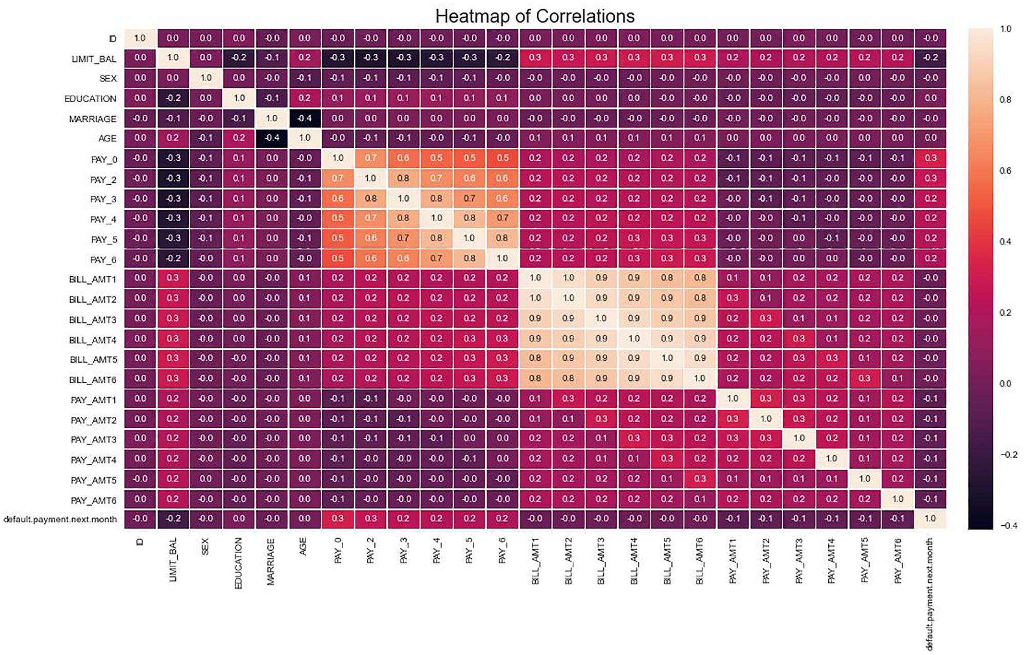
Data analysis
| Data set | Number ofsamples | Number ofpositive samples | Number ofnegative samples | Imbalancerate | Number of categories |
|---|---|---|---|---|---|
| Credit card | 30,000 | 6636 | 23,364 | 4.52 | 2 |
| Credit fraud | 284,807 | 492 | 284,315 | 577.88 | 2 |
Performance evaluation index
Experiment settings and results
Experiment settings
Group 1: (compare the feasibility of the proposed algorithm at different levels)
Group 2: (comparison between SEB-XGB and other imbalanced classification models)
Result analysis
| Data set | Evaluation index | Models | ||||
|---|---|---|---|---|---|---|
| XGBoost | SS-XGB | EE-XGB | SE-XGB | SEB-XGB | ||
| Credit card | AUC | 0.7545 | 0.7445 | 0.7645 | 0.7649 | 0.7728 |
| G-mean | 0.5763 | 0.6542 | 0.6933 | 0.6930 | 0.7003 | |
| Credit fraud | AUC | 0.9654 | 0.9683 | 0.9709 | 0.9740 | 0.9849 |
| G-mean | 0.8853 | 0.9078 | 0.9238 | 0.9364 | 0.9502 | |
| Data set | Evaluation index | Models | ||||
|---|---|---|---|---|---|---|
| RUSBoost | CatBoost | LightGBM | EBB-XGBoost | SEB-XGB | ||
| Credit card | AUC | 0.7623 | 0.7695 | 0.7687 | 0.7683 | 0.7728 |
| G-mean | 0.6874 | 0.5659 | 0.5674 | 0.7003 | 0.7003 | |
| Credit fraud | AUC | 0.9533 | 0.9685 | 0.9694 | 0.9821 | 0.9849 |
| G-mean | 0.9147 | 0.8738 | 0.8621 | 0.9344 | 0.9502 | |
| Data set | Parameter combination |
|---|---|
| Credit card | 0.1016, 5, 0.7701, 2.094, 0.9995, 90, 2.317, 2.187 |
| Credit fraud | 0.2999, 5, 1.5252, 0.5318, 0.8, 85, 0.0865, 1.5804 |
Conclusion
Declaration of conflicting interests
Funding
ORCID iD
Footnote
References
Cite
Cite
Cite
Download to reference manager
If you have citation software installed, you can download citation data to the citation manager of your choice
Information, rights and permissions
Information
Published In

Keywords
Rights and permissions
Authors
Metrics and citations
Metrics
Journals metrics
This article was published in International Journal of Distributed Sensor Networks.
View All Journal MetricsPublication usage*
Total views and downloads: 18138
*Publication usage tracking started in December 2016
Altmetric
See the impact this article is making through the number of times it’s been read, and the Altmetric Score.
Learn more about the Altmetric Scores
Publications citing this one
Receive email alerts when this publication is cited
Web of Science: 157 view articles Opens in new tab
Crossref: 203
- Predicting lithium-associated thyroid dysfunction through dimension reduction to establish a practical machine learning model: A retrospective multicenter study
- Tribological properties of non-equiatomic FeCoCrNiMn high entropy alloys: Molecular dynamics simulations and machine learning predictions
- Robust long-cable tension identification using XGBoost based on full-field vision recognition of multi-order mode shapes
- A Kriging-Markov hybrid method for real-time spatiotemporal indoor daylight prediction under data-sparse and sensor-limited conditions toward adaptive daylight control applications
- Proceedings of the 2025 6th International Conference on Computer Science and Management Technology
- Flow pattern prediction of gas/liquid two-phase flow over wide range of liquid viscosity and inclination angle using machine learning
- Reliable pneumonia detection and wheeze–crackle classification via data balancing and augmentation
- A Machine Learning-Based Spatial Risk Mapping for Sustainable Groundwater Management Under Fluoride Contamination: A Case Study of Mastung, Balochistan
- Prediction of Endpoint Phosphorus Content in Converter Steelmaking Using K-means and Bayesian-optimized Stacking Ensemble Learning
- Quality assessment and control of urban environmental sensors using physical thresholding and machine learning-based probabilities
- View More
Figures and tables
Figures & Media
Tables
View Options
View options
PDF/EPUB
View PDF/EPUBAccess options
If you have access to journal content via a personal subscription, university, library, employer or society, select from the options below:
I am signed in as:
View my profileSign out

I can access personal subscriptions, purchases, paired institutional access and free tools such as favourite journals, email alerts and saved searches.
loading institutional access options
Alternatively, view purchase options below:
Access journal content via a DeepDyve subscription or find out more about this option.
