	New content
Advances in Mechanical Engineering

Open access

Research article

First published online October 24, 2023

The impact of curved-tip propeller geometry on hovering drone performance for air quality monitoring

Mohamed Abdessamia Chakchouk https://orcid.org/0009-0004-1415-9888 [email protected], Abdelkhalak El Hami, […], Pierre Richard Dahoo, Azzedine Lakhlifi, Wajih Gafsi, and Mohamed Haddar+3View all authors and affiliations

All Articles

https://doi.org/10.1177/16878132231206330

Abstract

The success or failure of a drone mission depend on several elements, including the drone’s mass and payload, the surrounding environment, the battery’s state, and the propulsion system’s performance. Several studies have been undertaken addressing the propeller performance of this final component, particularly for fixed-wing or quad copter drones with ducted propellers. However, the shape of propeller blades used on tiny civil drones has not drawn as much attention. In this research work, the performance characteristics of a 10 × 4.7-inch curved tip propeller were explored, with the Advanced Precision Composite drone propeller serving as a design reference. This study seeks an alternative to ducted propellers when mass or size limitations prevent their use. The Computational Fluid Dynamics model was confirmed by comparing simulation results to the experimental propeller data source established by the University of Illinois at Urbana-Champaign, starting with a standard type propeller and using thrust coefficient as the key performance indicator. Moreover, the data analysis for the bended tip propeller replicating the well-established model, revealed the benefits as well as the drawbacks of such propellers on the mission profile and the battery lifespan of a quad copter Unmanned Air Vehicle.

Introduction

The performance of drones is significantly influenced by the design and operation of their propellers, which impact crucial parameters such as efficiency, stability, maneuverability, and flight duration.^1,2 The aerodynamics of propellers, particularly the generation and management of propeller vortices, play a vital role in defining flight performance.³ However, these vortices can lead to reduced thrust, increased noise, equipment interference, and potential threats to the propulsion system’s integrity.^4,5

To enhance propeller performance, numerous strategies have been explored, including the use of ducts to mitigate propeller noise. However, this approach has inherent constraints.⁶

Insightful numerical investigations by Mi⁷ have highlighted the significant influence of environmental factors, such as ground, sea surface, and wave conditions, on the aerodynamic properties of ducted propellers. Extensive research efforts have focused on optimizing ducted fan efficiency and stability through flow control techniques and innovative configurations.⁸ This emphasizes the critical interplay between propeller design and external environmental conditions.

Comparative studies have been conducted to assess the aerodynamic performance of contra-rotating ducted fans and open contra-rotating fans researchers, such as Akturk and Camci,^9,10 have provided valuable insights into the complex flow field dynamics during hovering and crosswind operations. Chen et al.¹¹ have emphasized the need for further innovation in ducted propeller design, particularly for hovering tasks. Their inventive design incorporating a tip jet for VTOL aircraft has demonstrated enhanced blade thrust, albeit with an increased overall weight.

The use of ducted propellers in high-speed forward flight presents challenges due to increased drag.¹¹ Pitching moment and architectural constraints affect their stability and overall system efficiency.¹² Proximity effects, such as ground effect, can induce rotational stall phenomena and reduce flow rate.¹³ Tip clearance and the number of blades in a propeller are additional design considerations that impact performance.^14–24 The use of ducts is then limited in certain circumstances, researchers aim in this case to improve the performance of the propeller system otherwise. Optimizing propeller shape, including chord length, pitch angle, twist, sweep, and lean, is crucial for efficient and high-performance propellers.^25–31 Studies have demonstrated the impact of these design elements on propeller efficiency, pressure ratio, and structural performance.²⁸ Spiroid winglets have shown potential in reducing wingtip vortices and improving aircraft efficiency.^32–34 High aspect ratio wings have been favored for their reduced induced drag.³⁵

To fill this research gap, our study conducts a groundbreaking investigation into the performance of a 10 × 4.7-inch propeller with curved tips, a design inspired by the marine industry’s Kappel propeller and modeled after the widely used APC drone propeller. This propeller design has not been thoroughly investigated within the context of drone applications. The implications of the modified shape on the overall drone performance are then examined. By scrutinizing the aerodynamic performance of the bended tip propeller, this study aspires to enrich the collective understanding of propeller design for drones, thereby laying the groundwork for further advancements in this domain.

Background

To determine lift and torque of a propeller, the simple blade element theory suggests calculating the aimed physical quantities for each of these elements and then summing them. This theory demonstrates the significance of each element in the propeller’s geometry as a fundamental aspect of its efficiency.³⁷ Since the propeller blade will be set at a given geometric pitch angle (β), the local velocity vector will create a flow angle of attack on the section. In this respect lift and drag components normal to and parallel to the propeller disk can be calculated so that the contribution to thrust and torque of the complete propeller from this single element can be obtained.³⁷

The difference in angle between thrust and lift directions is defined as:

ϕ = β - α

(1)

The elemental thrust and torque of this blade element can thus be expressed in terms of:

Δ T = Δ L \cos (ϕ) - Δ D \sin (ϕ)

(2)

\frac{Δ Q}{r} = Δ D \cos (ϕ) + Δ L \sin (ϕ)

(3)

The operation of a propeller can be handled using the same physical principles as that of a wing. The propeller has air moving around the top and bottom, creating a high-pressure zone and a low-pressure zone.

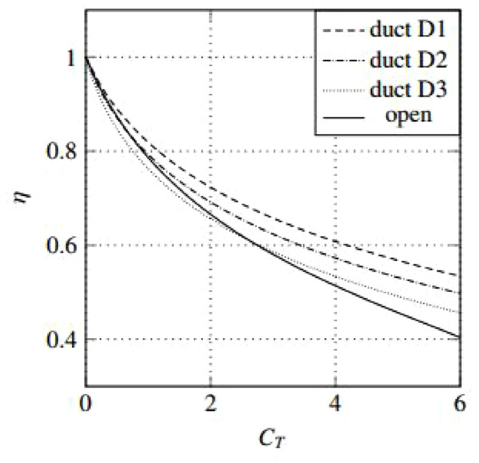
The most common practice to enhance propeller performance is adding ducts, as portrayed in Figure 1. However, ducted propellers pose additional challenges for a drone, as good efficiency necessitates very small clearances between the blade tips and the duct. Its weight increases the overall weight of the drone and at high angles of attack, parts of the duct will stall and produce aerodynamic drag. Unless these problems are solved, the duct loses its main purpose and becomes unbeneficial to install. In fact, the more parts are added to a rotational structure, the more uncertainties are created. For this reason, racing drones do not rely on using ducts, which is the case for the special drone mission like “Ingenuity” that NASA sent to mars.

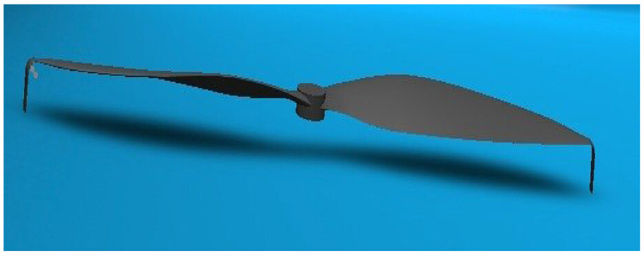
Figure 1. Ducted propeller and free propeller performance.³⁸

To find a descent substitute to the ducted propeller, the curved tip propeller will be discussed in this paper, as recorded in Figure 2. It corresponds to a promising technology that is utilized in the maritime area.^39–42 To some extent, the higher the bend angle is, the greater the reduction in propeller drag.⁴¹ Curved-Tip propellers, as opposed to ducted, tandem, or contra-rotating propellers, may respond suitably to these requirements. A simple technique to enhance propulsive efficiency is to shift the span wise load distribution toward the propeller tip. The Kappel propellers, used in the maritime transport field, adopt a similar approach. In this case,^43–45 the “endplate” is a continuous piece of the blade rather than an extra foil at the tip, and it effectively points toward the suction side (as with aircraft winglets).

Methodology

The starting point for our analysis was the selection of the conventional APC slow flyer propeller, specifically the 10 × 4.7-inch variant. This propeller served as a benchmark for comparison and provided a reference point for evaluating the performance of the modified design. To determine the appropriate motors for our study, we utilized a surrogate model developed with SCILAB. The surrogate model was crucial in modeling the flight plan and ensuring drone stability. From the stability analysis viewpoint described in our previous work,^46,⁴⁷ we derived the range of rotational speeds that the propellers could achieve. By analyzing the data, for each suggested propeller type we identified the propeller with the RPM range best supported by the chosen motors. The CFD analysis model was established in two stages. Firstly, using the conventional APC propeller, we selected the thrust coefficient as the primary performance criterion to validate the numerical setup accuracy by comparing the results with those found in Illinois database.³⁶ This step allowed us to ensure the reliability and consistency of our CFD performed using ANSYS Fluent 20 R1.

In the second part of the study, we optimized the propeller design by curving the tips by 90°, using SOLIDWORKS software to help reduce vortices. To assess the performance of the modified propeller design, we replicated the validated CFD analysis using the same parameters, but with the modified propeller design. We focused on evaluating the propeller’s aerodynamic performance and its impact on the flight time duration and the maximum payload capacity. This was done by coupling the Ansys fluent simulation data to a developed MATLAB algorithm that calculate these quantities based on the given equation listed in the end of the discussion.

Numerical setup

Flow domain

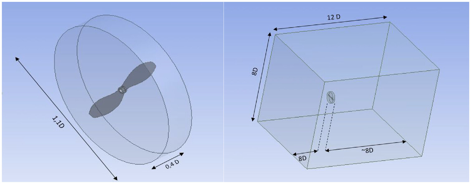
Before starting the simulation, the stationary domain’s inlet, outlet, and boundary were stretched to guarantee that the flow is completely developed as it enters and departs from the simulation domain. The intake boundary was eight times the diameter D from the propeller’s origin and the outlet boundary. The enclosure was set, as foregrounded in Figure 3, to 1.1 D for the rotating domain and to 0.4 D for the stationary and rotating domains, respectively.

Mesh generation

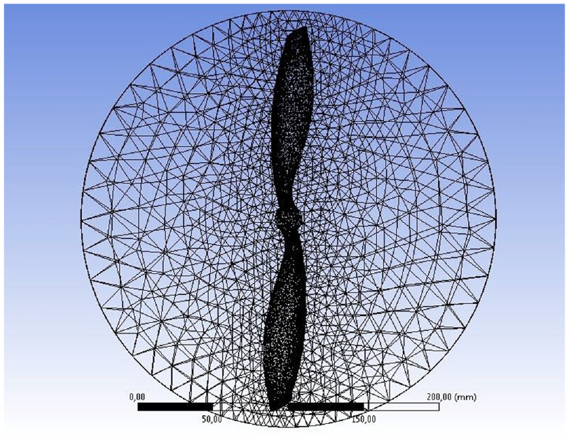
The flow field of the propeller was stationary in the rotating coordinate system. The ANSYS FLUENT CFD physics preference was used to settle the problem. To discretize the governing equations, the finite volume method with a pressure-based solver was applied. The grid was fully tetrahedral in both the rotating and static zones, as depicted in Figure 4. Tetrahedral elements fitted arbitrary shaped geometries very well with their simple computations so as to reduce the cost of computation.

Engineers frequently aim for 15–30 inflation layers (N = 15 to N = 30) through the thickness of the boundary layer when creating the mesh for turbulence modeling. Turbulence modeling for aerodynamic flows using Reynolds-averaged Navier-Stokes (RANS) was carried out on a single sheet of material rather than numerous layers, as illustrated in the instance above.⁴⁸

Re = \frac{ρ UL}{μ}

(4)

The Reynolds number gives a measure of the ratio of inertial forces to viscous forces and can be used to determine if a flow will be laminar or turbulent, where ρ is the fluid density, U is the freestream velocity, L is the geometry’s characteristic length, and µ dynamic viscosity of the fluid. The skin friction coefficient was then estimated using an equation that specifies out how much friction there is on a given surface.³⁷

C_{f} = {[{2 \log}_{10} (Re) - 0.65]}^{- 2.3}

(5)

After calculating the skin friction coefficient, the wall shear stress (w) was determined in terms of

τ_{w} = 0.5 * ρ U^{2} C_{f}

(6)

The

y^{+}

equation can be tweaked to get the height of the wall next cell centroid from the wall (

y_{p}

), yielding

y_{h}

. The cell’s height

y_{h}

is twice the value of

y_{p}

, and the distance between the cell centroid and the wall is

y_{p}

⁴⁹;

y^{+} = \frac{ρ y_{p} u_{t}}{μ}

(7)

y_{h} = 2 y_{p}

(8)

As the skin friction coefficient was calculated empirically for each flow situation, the starting cell height provided by these equations provided only an approximation. In real-world CFD calculations, skin friction coefficients are anticipated to be comparable, but not identical, to those of a flat plate. Resting on this calculation, the element size criteria were imposed as 3e-3 on the surface of the propeller. An adaptive sizing was implemented on the stationary domain and the growth rate was fixed at 20%. The inflation was set to be program controlled with a smooth transition.

There are several criteria that need to be met before a mesh can be considered acceptable for CFD study, including initial cell height, growth ratio, and ultimate layer height. The user has additionally to examine the mesh quality metrics as well as the overall level of resolution in locations of interest. These requirements differ from case to case and necessitate an examination on a case-by-case basis. Table 1 exhibits the details for the mesh grid. It is noteworthy that standard meshing is more suitable for this type of problem.

Table 1. Mesh quality parameters.

Mesh metric	Minimal value	Maximal value	Average
Element quality	5.402e-002	1	0.82935
Skewness	8.605e-006	0.97	0.24
Aspect ratio	1.1594	31.06	1.8701

Boundary conditions

In the solver’s setup definition, an absolute frame was used. In fact, since the rotating zone walls were separated from the static zone walls, much of the flow away from the propeller would have a low velocity. The turbulence intensity amounted to 0.1% on the inlet, and slip condition was imposed. It indicates that the fluid adheres to the wall and moves at the same velocity as the wall, if it is moving. This is the case in our study because the static zone walls were spaced far enough apart to ensure this condition.

An MRF was assigned to the propeller’s rotating domain to account for the rotational movement of the grid cells. MRF simulations required far less computational power than transient modeling. As a result, if the problem is properly set up, MRF can provide good approximations while requiring less computational effort and time. The rotating zone propeller wall was also assigned a rotational designation. Using a Semi-Implicit Method for Pressure-Linked Equations, the pressure–velocity coupling was accomplished. For velocity and pressure, the Second Order Upwind method was applied. The gradients were computed using the Least Square Cell-based Algorithm as well as the second Order Upwind for Turbulent Kinetic Energy and Turbulent Dissipation Rate.

The two-eq9 models k-ε and k-ω models present a general description of turbulence through two transport equations. One for the turbulence kinetic energy k and the other for the specific turbulence dissipation rate ω. They all rely on Boussinesq’s approximation from 1877, where the stress tensor is modeled in the viscous term of Navier-Stokes Equation. As far as our simulation is concerned, the standard k-e model, requiring a fully turbulent flow, was used to simulate turbulence. The convergence was also ensured through monitoring the residual value as it falls below a certain threshold. This would be an indicator of a mathematical solution implying that the simulation was able to stabilize. However this means on the other side only a mathematical convergence, as monitoring physical parameters such as force, drag, or average temperature might help the users determine whether their study yielded a feasible solution.⁴⁹

Results and discussions

The force and momentum of a propeller were resolved in a three-coordinate system with the parameters x, y, and z, where T (N) is thrust, Q (N m) is torque, n (rps) is propeller rotational speed per second, d (m) is diameter, and ρ is fluid density. Both the thrust coefficient, C_T, and the torque coefficient, C_Q, have a relative percentage error. The numerical analysis results were compared to available experimental data so as to confirm the grid’s influence.¹

Δ = \frac{{C_{T}}_{CFD} - {C_{T}}_{EXP}}{{C_{T}}_{EXP}} * 100

(9)

C_{T} = \frac{T}{ρ n^{2} D^{4}}

(10)

Results

In the solution method task page, the SIMPLE resolution method uses a relationship between velocity and pressure corrections to ensure mass conservation and to obtain the pressure field. In addition, for the transient algorithm, a second order implicit formulation was used. Second order algorithms entail the greatest results since they decrease interpolation mistakes significantly. Furthermore, the simulation was then initiated with 1e-006-time steps and 100 iterations by time step. In this approach, higher-order accuracy was achieved at cell faces through a Taylor series expansion of the cell-centered solution about the cell centroid, with a slower convergence.

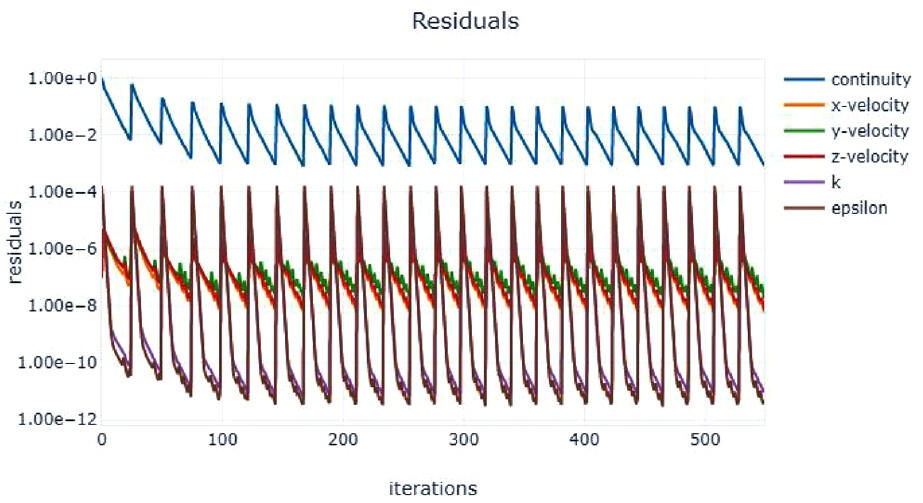
In a CFD analysis, the residual measures the local imbalance of a conserved variable in each control volume. Every cell in your model is assigned its own residual value for each of the equations being solved.

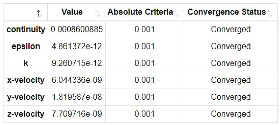
For CFD, RMS residual levels of 1E-4 are considered loosely converged, while 1–5 is regarded well converged and 1–6 is considered tightly converged. Figure 5 illustrates a screen shot from the Ansys fluent report, Figure 6 shows the status of convergence for all the residuals.

Figure 6. Status of convergence for the residuals.

For complicated problems, however, it’s not always possible to achieve residual levels as low as 1E-6 for a simple problem. In our simulation, the achieved residuals are as low as 1E-6.

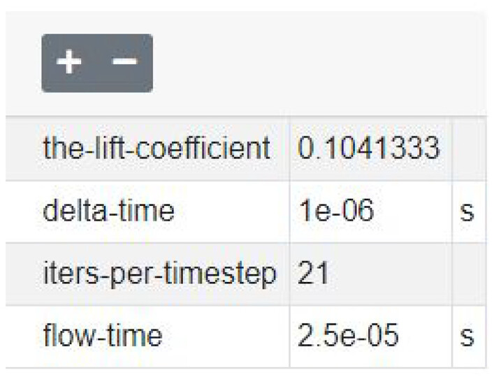
For an analysis to be called converged, the solution field should not fluctuate from an iteration to an iteration. In our board design, the drag and the lift can be invested as monitor points in the experimental as well as in the simulation studies. In our case, the lift coefficient was chosen as the physical monitor. The corresponding solution yields stable progression of results when changing RPM. The pattern of the thrust coefficient was stabilized with minimum computational cost, as shown in Figure 7.

The experimental data from data source created by the University of Illinois at Urbana-Champaign were used to assess the results found by the CFD analysis. As provided in Table 2 and Figure 8, the first simulation was conducted for 2500 RPM speed .The result provided in the ansys fluent is outlined in Figure 8.

Table 2. CT from cfd and CT from experiments.

Speed	CT cfd	CT exp
2500	0.1041	0.1039
3000	0.091	0.1100
3500	0.0915	0.1117
4000	0.0914	0.1158
4500	0.094	0.12
5000	0.096	0.1237

Figure 8. Static thrust coefficient for 2500 RPM.

The now-selected model was copied, and the propeller’s shape was modified using Solidworks 2020 to bind the tips. Our major target lies in designing curved tips that mimic the intersection of the propeller and the commonly used duct in these situations. After bending the tips in Solidworks, we proceeded with a geometry correction using the ansys space claim tool to eliminate miscreated corners, fuse surfaces, and point out the problematic geometries, after which the modified propeller will be injected in the duplicated model by simply replacing the old one. The meshing sizing was also determined using the same method as the previous simulation and retaining the same meshing parameters. 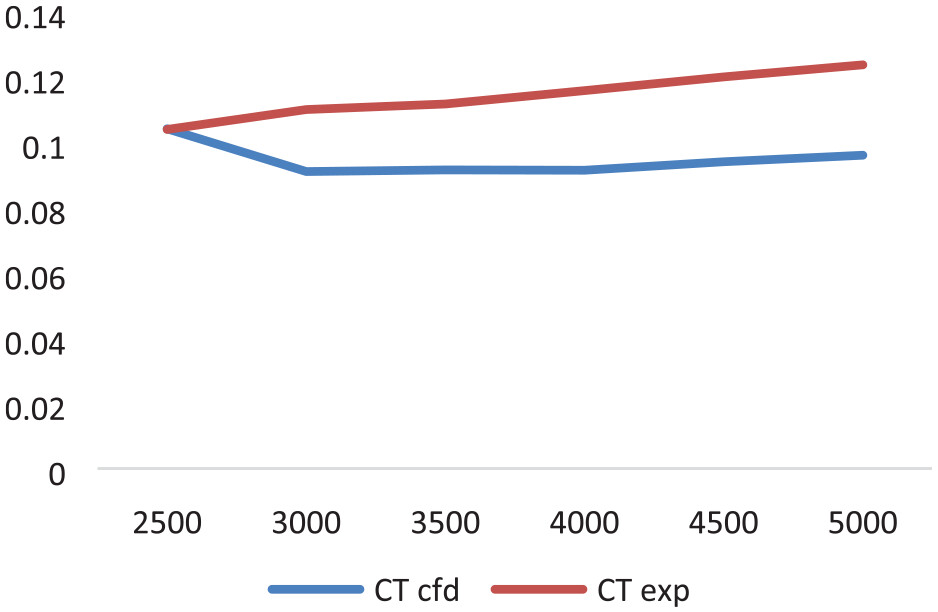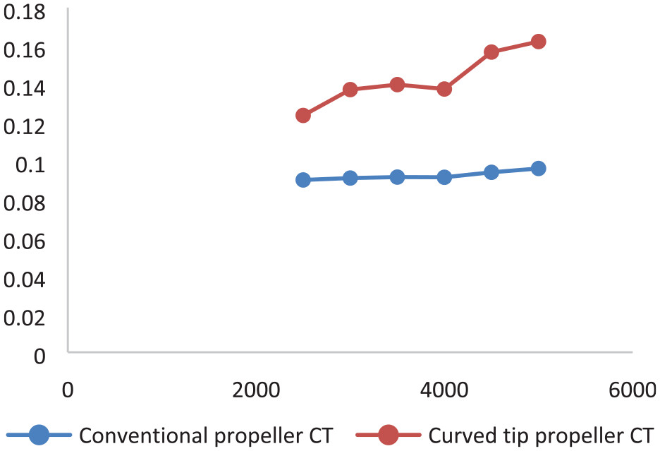Table 3 and Figure 9 as well as Figure 10 illustrate the CT difference between conventional type and curved type propeller.

Table 3. Thrust coefficient from conventional propeller and curved tip propeller for static performance.

Speed	Conventional propeller CT	Curved tip propeller CT
2500	0.1039	0.1237
3000	0.1100	0.1372
3500	0.1117	0.1398
4000	0.1158	0.1375
4500	0.12	0.1568
5000	0.1237	0.1623

Figure 9. Comparison from CT from cfd and CT from experiments.

Figure 10. Comparison between thrust coefficient from conventional and curved tip propeller.

At this stage of analysis, using an advance ratio J to simulate the flying state by imposing an air speed in the inlet from j is indicated by the formula J =

\frac{V}{n * D}

. The results suggest that the curved-tip propeller has a better thrust for the vast majority of j.

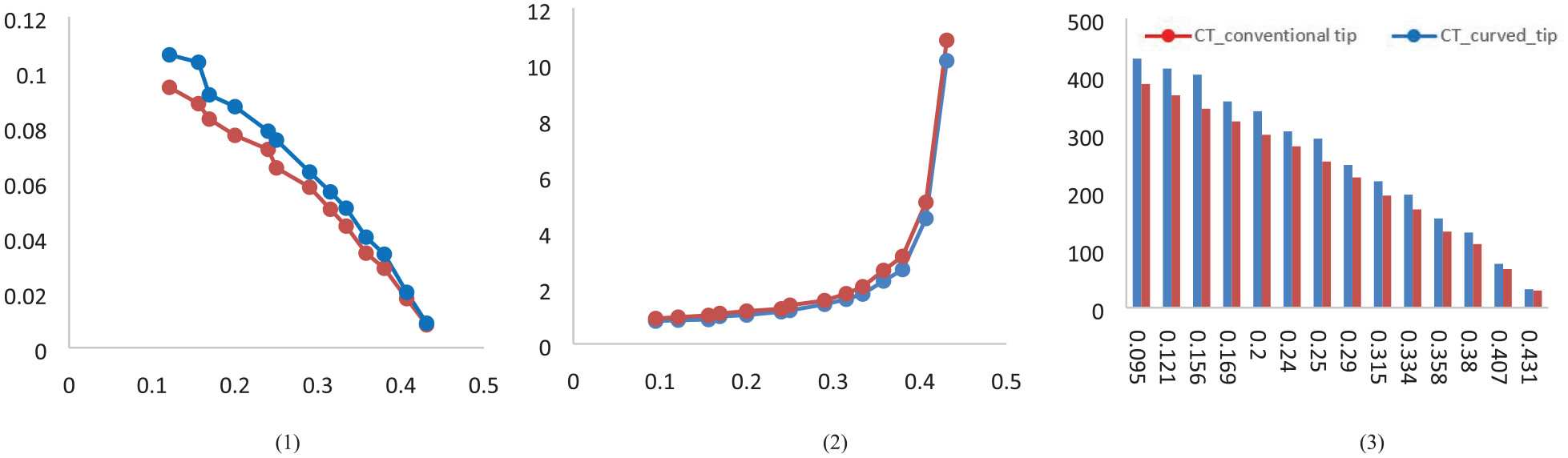
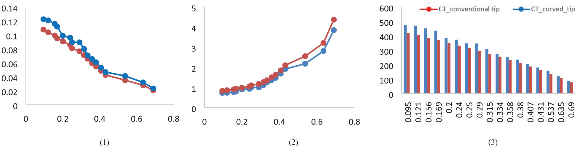
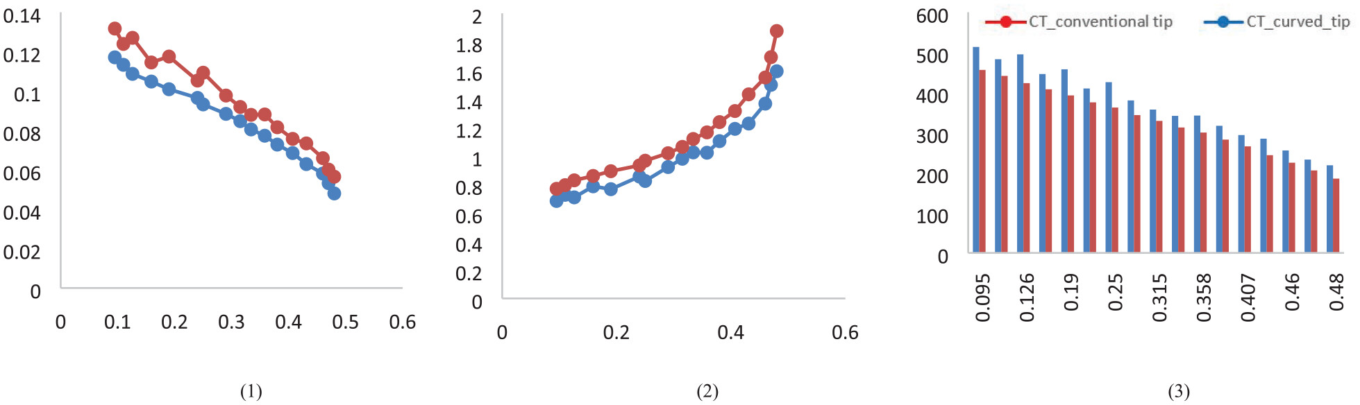
A key parameter of interest is the thrust coefficient (Ct), which encapsulates the efficiency of the propeller design. The drone’s flight time (T) and its payload carrying capacity are critically dependent on this coefficient they are calculated by coupling ansys fluent results to a developed MATLAB algorithm results are illustrated in Table 4 and represented with Figure 11 for 4000 RPM, Figure 12 for 5000 RPM, and Figure 13 for 6000 RPM.

Table 4. Effect of thrust coefficient on flight time and payload capacity: a comparison between conventional and curved tip propellers.

J	CT_conventional tip	CT_curved_tip	Flight time modified	Flight time conventional	Max payload curved tip	Max payload conventional tip
4000 RPM
0.1	0.0994	0.1106	0.814	0.905	430.662	386.747
0.2	0.0944	0.1062	0.847	0.953	413.410	367.142
0.2	0.0885	0.1035	0.869	1.017	402.823	344.008
0.3	0.0829	0.0917	0.981	1.086	356.555	322.050
0.3	0.077	0.0874	1.03	1.169	339.695	298.916
0.3	0.0719	0.0785	1.146	1.252	304.798	278.919
0.4	0.0652	0.0753	1.195	1.380	292.251	252.649
0.4	0.0582	0.0637	1.413	1.546	246.767	225.202
0.4	0.0502	0.0565	1.593	1.793	218.536	193.834
0.5	0.0441	0.0506	1.779	2.041	195.402	169.916
0.5	0.0343	0.0401	2.245	2.624	154.232	131.490
0.5	0.0288	0.0339	2.655	3.126	129.921	109.924
0.6	0.0178	0.0201	4.479	5.058	75.8120	66.793
0.6	0.0083	0.0089	10.116	10.84	31.896	29.544
5000 RPM
0.1	0.1077	0.1225	0.734	0.835	477.322	419.291
0.1	0.1038	0.1209	0.744	0.867	471.048	404
0.2	0.0993	0.1161	0.775	0.906	452.227	386.355
0.2	0.0953	0.112	0.803	0.944	436.151	370.67
0.2	0.0908	0.0988	0.911	0.991	384.394	353.026
0.3	0.0856	0.0961	0.936	1.051	373.808	332.637
0.3	0.0811	0.0896	1.004	1.110	348.321	315
0.3	0.0766	0.0894	1.007	1.175	347.537	297.348
0.4	0.0709	0.0799	1.126	1.269	310.287	275
0.4	0.066	0.0708	1.271	1.364	274.606	255.785
0.4	0.0597	0.0656	1.372	1.508	254.217	231.083
0.4	0.0549	0.0608	1.480	1.639	235.396	212.262
0.5	0.0486	0.0532	1.692	1.852	205.597	187.560
0.5	0.0428	0.0468	1.923	2.103	180.50	164.818
0.5	0.0352	0.0413	2.180	2.557	158.937	135.011
0.6	0.028	0.032	2.813	3.215	122.471	106.787
0.6	0.0206	0.0234	3.847	4.370	88.751	77.68
6000 RPM
0.1	0.1171	0.1317	0.683	0.768	513.395	456.148
0.12	0.1133	0.1239	0.726	0.794	482.811	441.249
0.15	0.1087	0.127	0.708	0.828	494.966	423.212
0.17	0.1048	0.1145	0.7863	0.859	445.954	407.920
0.19	0.1009	0.1175	0.766	0.892	457.717	392.628
0.22	0.0965	0.1053	0.855	0.933	409.881	375.376
0.24	0.0932	0.1093.	0.823	0.966	425.565	362.437
0.27	0.0884	0.0977	0.921	1.018	380.081	343.616
0.29	0.0847	0.0919	0.097	1.062	357.337	329.108
0.32	0.0805	0.0879	1.024	1.118	341.655	312.640
0.33	0.0773	0.0881	1.021	1.164	342.440	300.093
0.36	0.0728	0.0816	1.103	1.236	316.953	282.448
0.38	0.0685	0.0757	1.189	1.314	293.819	265.588
0.41	0.0629	0.0734	1.226	1.431	284.801	243.630
0.43	0.0581	0.0659	1.366	1.549	255.393	224.810
0.45	0.0532	0.0601	1.490	1.692	232.652	205.597
0.48	0.048	0.0565	1.593	1.875	218.536	185.207

Figure 11. Comparison between curved tip propeller and conventional tip propeller for 4000 RPM: 1 – thrust coefficient, 2 – flight time duration, 3 – maximum payload.

Figure 12. Comparison between curved tip propeller and conventional tip propeller for 5000 RPM: 1 – thrust coefficient, 2 – flight time duration, 3 – maximum payload.

Figure 13. Comparison between curved tip propeller and conventional tip propeller for 6000 RPM: 1 – thrust coefficient, 2 – flight time duration, 3 – maximum payload.

Discussions

Using the data summarized in Table 4, our analysis compared conventional and curved propellers, where the curved propeller exhibited a 15.9% higher average Ct and 6.1% greater maximum payload capacity. However, the flight time for drones with curved propellers was approximately 6.7% lower than for those with conventional propellers. Indeed, the relationship between thrust coefficient and thrust is represented by equation (10).

Referring to the prevalence of Li-Po cells and batteries in commercial UAVs, they were utilized for these computations. The energy consumption calculation was largely based on the information cited in the bibliography for the vertical upward energy consumption.^50,⁵¹ The amount of energy used from the battery grows as the time of takeoff for flights at higher altitudes increases.

The formula that links the thrust and the weight is determined as⁵²

F_{t, v} = M_{tot} g + \frac{1}{2} ρ A_{t} C_{d} V_{v}^{2} = M_{tot} g + \frac{1}{2} ρ A_{t} C_{d} V_{v}^{2}

(11)

For this mission profile, the drone will be hovering for most of the flight. Therefore, we may disregard the vertical speed

V_{V}^{2}

. The thrust is hence a function of mass alone, and the gain is transferred to the overall weight of the payload. Notably, the increase in thrust will need additional power to be supplied, as thrust and power are closely connected by this equation⁵³

P = \sqrt{\frac{F^{3}}{2 ρ A_{p}}}

(12)

This increase is automatically indicative of an increase in the average amperage draw specified by:

AAD = AUW * P / V

In our case study, the needed power with the new topology was multiplied by 14. Thus, if we chose to install this modified propeller with the same batteries, we would have a time of flight^47,53 expressed by equation (13):

T' = capacity \times discharge / AAD'

(13)

T' = capacity \times discharge / [(AUW * P') / V]

The results emphasize the trade-off between thrust coefficient, flight time, and payload capacity, highlighting the need for optimizing propeller design for lift generation and energy efficiency. The most promising aspect of this type of propellers is their potential to accommodate greater payloads while maintaining the same size. Future research should focus on advanced propeller shapes and materials to achieve a balance between these factors.

Conclusion

This study presents a simulation of an altered propeller shape using a CFD model developed on ANSYS fluent to investigate its performance. The choice of the propeller type is based on a SCILLAB simulation presented in Chakchouk et al.⁴⁷ As for the verification and validation of the CFD model, we invested the APC propeller data set developed by University of Illinois at Urbana-Champaign. The convergence study of the solution was monitored both mathematically and physically, opting for the thrust coefficient as the main monitor.

This study is, to the best of our knowledge, the pioneer investigation of a curved tip propeller employed on a drone addressing its merits and deficiencies on the mission profile. The computational trend under static or forward flying conditions over the whole range of advance ratios (j) values indicated the performance advantage that may be achieved employing curved tip propellers. Results revealed that an estimated 25% increase in thrust force can be reached, which translates a capability for hovering to lift a load heavier than the initial load intended with the selection of the same propeller when it is conventional, yielding a more capable propeller with the same dimensions. However, the increase of thrust has a negative impact on the drone’s flying duration, which was shortened by 30%.

This shortcoming can be mitigated by cooperative task assignment of multi-UAV system. Besides, future study will explore the optimization of the other components of the system, such as the drone chassis and landing gear, motivated by the promising characteristics of this topology.

Declaration of conflicting interests

The author(s) declared no potential conflicts of interest with respect to the research, authorship, and/or publication of this article.

Funding

The author(s) disclosed receipt of the following financial support for the research, authorship, and/or publication of this article: This work was done in a collaboration between the LMN laboratory of INSA Rouen Normandie and the LATMOS laboratory of the University of Versailles St-Quentin Paris-Saclay, in support by LA2MP laboratory of Sfax and we thank all of these institutions for support. Fruitful discussions with Doctor Hichame Maaname are greatly acknowledged.

ORCID iD

Mohamed Abdessamia Chakchouk https://orcid.org/0009-0004-1415-9888

Footnote

Handling Editor: Chenhui Liang

Appendix

List of symbols, acronyms, and abbreviations

FTIR Fourier Transform Infrared

CFD Computational Fluid Dynamics

APC Advanced Precision Composites

UAV Unmanned Aerial Vehicle

SCILAB Scientific Laboratory

RPM Revolutions Per Minute

ANSYS Analysis Systems

CAD Computer-Aided Design

RANS Reynolds-Averaged Navier-Stokes

MRF Multiple Reference Frame

RMS Root Mean Square

CD Coefficient of Drag

Ct Coefficient of thrust

Li-Po Lithium Polymer

AUW All-Up Weight

V Voltage

AAD Average Amperage Draw

References

1. Bergmann D, Denzel J, Pfeifle O, et al. In-flight lift and drag estimation of an unmanned propeller-driven aircraft. Aerospace 2021; 8: 43.